Arithmetization-oriented ciphers are symmetric ciphers optimized for an advanced cryptographic protocol such as multi-party computation or zero-knowledge proofs.
Latest News
Stay up to date with the latest news by reading our blog posts.
This note discusses lattice-based cryptography over the field with $p = 2^{64}-2^{32}+1$ elements, with an eye to supporting lattice-based cryptography operations in virtual machines such as Miden VM that operate natively over this field. It discusses how to support Dilithium and Falcon, two lattice-based signature scheme recently selected by the NIST PQC project; and proposes parameters for efficient public key encryption and publicly re-randomizable commitments modulo $p$.
The project about algebraically cryptanalyzing AOCs has run its course. As is usually the case in research, there are a lot more questions left to answer. I have listed some of the more interesting ones below – if you are looking for inspiration, this might be a starting point.
The most pressing question is to find lower complexity bounds for Gröbner basis computations.
A polynomial system gives rise to various similar but distinct concepts in trying to capture the complexity of a Gröbner basis computation – for example the Hilbert Regularity1, the First Fall Degree, the Solving Degree, and others. Systematizing and relating the different definitions and concepts would greatly reduce confusion, helping not only newcomers but also experts.
It is generally assumed that computing a Gröbner basis for a polynomial system without any underlying structure is about as hard as it can get. Discovering structure, for example of a weighted homogeneous kind, then using the appropriate monomial order for computing the Gröbner basis, might speed up the computation. It is unknown how to discover structure like this.
It might be possible to divide a Gröbner basis attack for a keyed primitive into an offline and an online phase. In the offline phase, the plaintext and ciphertext are left as a variable, and the ideal of the polynomial system is of positive dimension. In the online phase, the acquired plaintext and ciphertext are plugged into the pre-computed Gröbner basis, and the key is derived. The details, feasibility, and overhead of such an approach are unclear.
Gröbner basis algorithm F5 has shown that the complexity of computing a Gröbner basis for a given set of polynomials can be characterized by the syzygy module for that set. It is believed that computing the syzygy module is as hard as computing the Gröbner basis, but whether this is actually the case is unknown.
Furthermore, it would be interesting to know if we can derive a polynomial system’s degree of regularity2 given its syzygy module.
AOCs use MDS matrices to mix the different state elements. Computing a Gröbner basis for the cipher can be seen as an unmixing of these transformations. It might be possible to incorporate an AOC’s MDS matrix3 into the monomial order to counteract the mixing.
There a bunch of open questions surrounding the Gröbner Walk. Can we find an upper bound on the number of cones in the Gröbner fan? (How) does the number of cones relate to the size of the staircase? Is the shape of the fan characteristic for a certain cipher? How does its performance to FGLM compare on systems derived from an AOC? Can we estimate the fastest path to one of the lex orders?
Many more questions regarding Gröbner bases still don’t have an answer, but this list has probably raised enough questions for a few years worth of research.
When estimating the security of a cipher or hash function, there are many different attack scenarios to consider. For Arithmetization Oriented Ciphers (AOCs), Gröbner basis attacks are a lot more threatening than they are to “traditional” ciphers, like the AES. The most common way to argue resistance against Gröbner basis attacks is to look at the expected complexity of Gröbner basis algorithms.
However, the complexity estimates only apply asymptotically, and the Big O notation might hide factors that are significant for parameter sizes a cipher designer is interested in. Thus, to validate whether the theoretical complexity estimates carry significance, we need “real” data to compare it to. This means running experiments – and that’s exactly what this post is about. Concretely, we have performed several Gröbner basis attacks, and will be discussing and interpreting the resulting data here.
Disclaimer
Take below results with a grain of salt – the data might be wrong. As far as I know, no one has reproduced it yet.1 Please draw any conclusions carefully.
Prerequisites
We assume a certain familiarity with the ciphers Rescue-Prime [4] and Poseidon [3], as well as the Sponge construction. As a quick reminder for these three things, there are graphical depictions at the end of this post and in the next section, respectively.
Since this post is all about Gröbner basis attacks, a certain familiarity on this topic does not hurt, albeit it shouldn’t be strictly necessary. In case you want to brush up on a detail or two, have a look here.
Description of Experiments
AOCs like Rescue-Prime and Poseidon are designed to have a “small” algebraic description. That is, when polynomially modeling their structure, we don’t need too many polynomials, and those are not of very high degree.
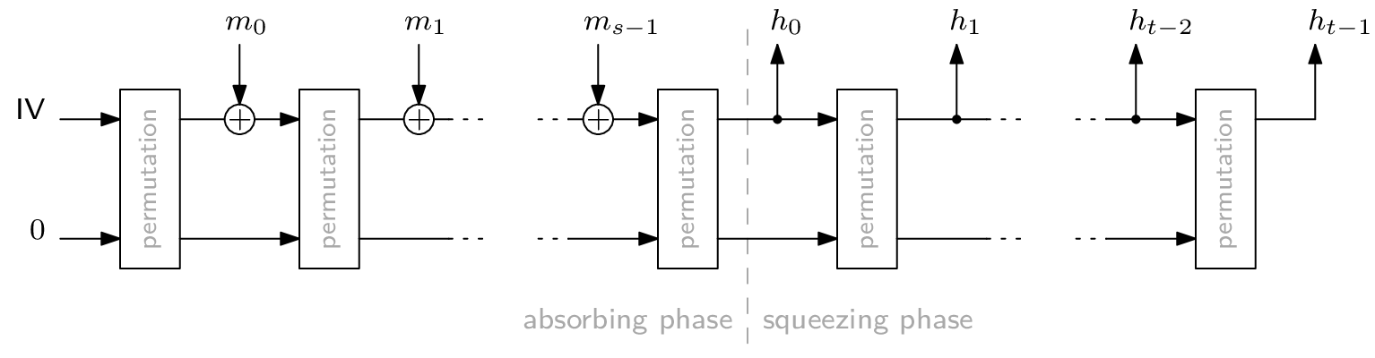
A use case where an AOC’s simple algebraic description causes major speedups involves hashes in zero-knowledge proof systems. The most popular way to transform a permutation, like Rescue-Prime or Poseidon, into a hash function is the Sponge construction. On a high level, a Sponge looks like this:
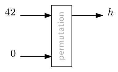
Any cryptographic hash function needs to be secure against inversion, i.e., computing a pre-image for a given hash digest must be so difficult as to be infeasible. For the Sponge construction, this largely depends on the plugged-in permutation. For our experiments, we perform a second pre-image Gröbner basis attack on a Sponge construction with exactly one application of the permutation. Furthermore, we set $\textsf{rate} = \textsf{capacity} = 1$, which is the lowest meaningful value for either parameter. This way, we get the smallest Sponge one can build. Consequently, if this attack is infeasible, then Gröbner basis attacking a realistically sized Sponge definitely is.
As the permutation, we use the two primitives Rescue-Prime and Poseidon with varying numbers of rounds. The prime field has size $p = 65519$, which is the largest 16-bit prime for which $\gcd(p-1, 3) = 1$, meaning we can use exponent $3$ in the S-Boxes.2 The limitation to 16-bit primes comes from the used Gröbner basis computation implementation, namely FGb [2].
Technical specifications
All the experiments were performed using cocalc on an “n2-highmem-32 Cascade Lake Google Compute Engine” and 264141536 KiB (~252 GiB) of total RAM as reported by free. The operating system in use was (Ubuntu) Linux 5.4.0-1042-gcp x86_64 as reported by uname -srm.
Reproducibility
The code for the experiments can be found on github. Its dependencies are sagemath, fgb_sage, and FGb [2]. If you have the abilities and capacity to re-run the code to strengthen or refute the claims made here, I encourage you to do so.
Summary of Results
Before looking at the data in a little more detail, here’s a quick summary of some of my findings.
We managed to compute a Gröbner basis for 6 rounds of Rescue-Prime, but failed at 7 rounds.
Poseidon has a two types of rounds, which makes arguing about round limits a little more cumbersome. With the exception of one outlier, we could not break any partition totaling 11 rounds – see the matrix below.
Memory, not time, seems to be the most limiting factor.
The polynomial system for Poseidon appears to be irregular, in contrast to the authors’ implicit assumption. This directly affects the number of recommended rounds. For example, while Poseidon’s authors recommend $(8,9)$ rounds for $p=65519$ and $|\textsf{state}| = 2$, extrapolating the data here suggests that $(8,24)$ rounds might be necessary.
The interpolation for the degree of regularity for Rescue-Prime is different from the interpolation published with Rescue, but similar in principle. This difference might be explained by the use of Rescue-Prime as the permutation. Sadly, it neither validates nor refutes the authors’ claims.
Results in Detail
Experiments like the ones described above generate quite a bunch of data. We’re not gonna look at everything here, I just want to highlight some parts. If you want to start digging deeper, you can find the raw data at the end of this post.
The metric commonly used to estimate the complexity of a Gröbner basis computation is largely depending on the degree of regularity.3 This is not based on a totally rigorus argument, but it seems to be “good enough” in practice. Consequently, quite a bit of the following will be about the degree of regularity and the Macaulay bound.4 The Macaulay bound is an upper bound for the degree of regularity, and their values coincide if a polynomial system is a regular sequence.
In general, the successful attacks that took the longest time for the two primitives were 6-round Rescue-Prime, and (full=2, partial=9)-round Poseidon. They took around 34 and 73 hours, requiring roughly 75 and 228 GiB, respectively.
Rescue-Prime
We successfully computed a Gröbner basis for 6-round Rescue-Prime, but ran out of memory during the computation for 7-round Rescue-Prime.
Degree of Regularity
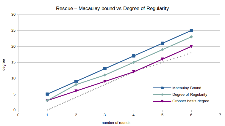
The most important metric to consider is the growth of the degree of regularity as a function in the number of rounds. As we can see, the degree of regularity is pretty consistently $2$ less than the Macaulay bound of the system for Rescue-Prime. The only exception happens at $r=2$ rounds, an anomaly I don’t believe deserves a lot of attention.
Interestingly, the degree of the highest degree polynomial in the resulting reducer Gröbner basis – abbreviated as the degree of the Gröbner basis – is even lower than that. More importantly though, its growth seems to be only piecewise linear: between 1 and 4 rounds, the degree of the Gröbner basis grows by $3$ with each iteration, where from round 4 on, the difference is $4$. The limited number of data points makes drawing conclusions difficult. However, it’s not unreasonable to argue that extrapolating the degree of the Gröbner basis linearly might lead to inaccuracies. Similarly, it is still an open question whether extrapolating the degree of regularity is a good method to estimate the complexity of computing the Gröbner basis for the full-round primitive.
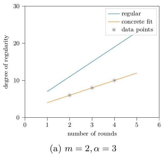
The observed growth of the degree of regularity in Rescue-Prime is different from what is reported in the publication of “plain” Rescue. Concretely, I observe $d_\text{reg} \approx 4r-1$ for Rescue-Prime, whereas Rescue’s authors report $d_\text{reg} = 2r+2$ for Rescue [1, Section 6.1]. Here is their figure for comparison:
Extending this interpolation of the degree of regularity to an extrapolation can be used to estimate the required number of rounds to achieve a given security level. For this, we use the known complexity bound for the most performant Gröbner basis algorithm, which is $\binom{n + d_\text{reg}}{n}^\omega$. Here, $n$ is the number of variables in the polynomial ring, $d_\text{reg}$ is the degree of regularity, and $\omega$ is the linear algebra constant. A conservative choice for $\omega$ is $2$. While there are no implementations of Gröbner basis algorithms making use of sparse linear algebra techniques that I know of, it is possible that they exist, or that they will exist at some point in the future. For the used parameters of Rescue-Prime, the number of variables, which is equal to the number of equations, is $2r$. The degree of regularity is estimated to be $4r – 1$. Putting it all together, we have $\binom{6r – 1}{2r}^2 > 2^{128}$ for $r \geqslant 13$. For the same parameters, the authors of Rescue-Prime recommend $r=27$ [4, Algorithm 7]. This recommendation also includes a security margin, and considers more attack vectors than just a Gröbner basis attack.
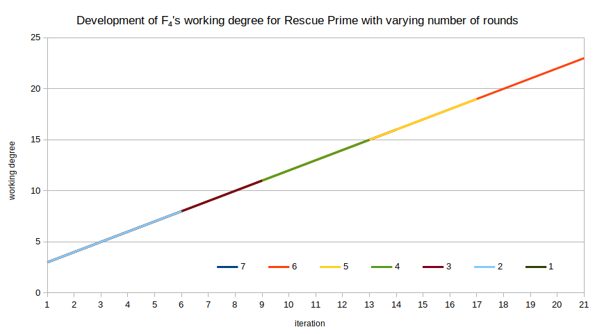
Working Degree
The working degree of F4 increases strictly monotonously: every iteration of F4‘s main loop means working with polynomials of degree exactly $1$ higher than in the preceding iteration. That makes for a pretty dull figure:
Poseidon
Since Poseidon has two types of rounds, namely full rounds and partial rounds, we have conducted a lot more experiments for Poseidon than for Rescue. The following matrix summarizes which ones we ran, and whether the Gröbner basis could be computed successfully. The value of a cell indicates how many polynomials the polynomial system had. This is equal to the number of variables in the polynomial ring for this problem instance. The number of full rounds differ across columns, the number of partial rounds across rows.
2
4
6
8
10
12
0
3
7
11
15
19
23
1
4
8
12
16
20
2
5
9
13
17
21
3
6
10
14
18
4
7
11
15
19
5
8
12
16
6
9
13
17
7
10
14
8
11
15
GB computed
9
12
16
out of memory
10
13
manually aborted
A total of $11$ rounds seems to the barrier we couldn’t break with the available machine, the (2,9)-instance being a notable exception. Note that the number of equations seems to not be the cutoff point – for (2,10)-Poseidon, we have 13 equations and variables but cannot compute the Gröbner basis, whereas for (10,0)-Poseidon with its 19 equations, we can compute the Gröbner basis. For some of the figures below, we look at the series for $r_\text{full} = 4$ full rounds in more detail to simplify presentation.
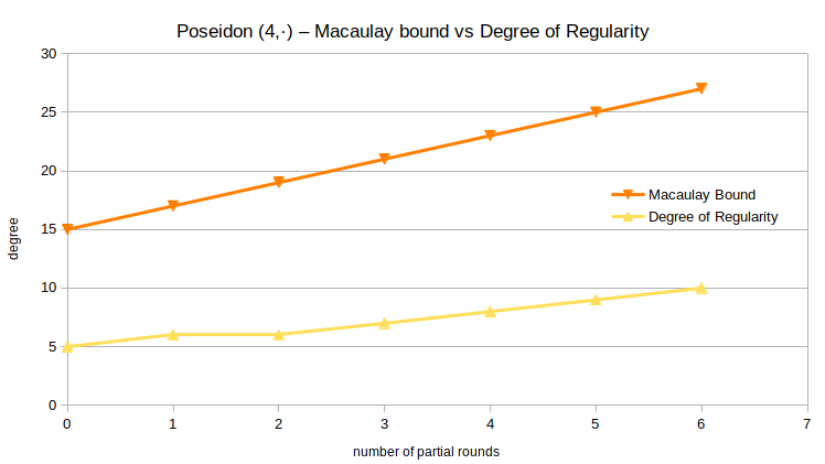
Degree of Regularity
As before, the degree of regularity is the metric we’re interested in the most. For example, for Poseidon (4,·), i.e., 4 full rounds and a varying number of partial rounds, we get the following figure when plotting both the Macaulay bound and the system’s degree of regularity.
It appears the degree of regularity is growing slower than the Macaulay bound. For a more complete picture, the degrees of regularity for all successfully computed Gröbner bases are listed in the following table. A grayed-out value means that the Gröbner basis computation did not terminate, but reached the indicated degree at its maximum before running out of memory or being aborted manually.
2
4
6
8
10
12
0
4
5
6
7
8
8
1
5
6
6
7
8
2
5
6
7
8
8
3
6
7
8
9
4
7
8
9
9
5
8
9
9
6
9
10
10
7
10
11
8
11
12
9
12
13
10
13
We can compute the Macaulay bound for the polynomial system arising from $(r_\text{full}, r_\text{partial})$-Poseidon as $4r_\text{full} + 2r_\text{part} – 1$. A closely fitting linear approximation for the degree of regularity based on above data is $d_\text{reg} \approx \frac{r_\text{full}}{2} + r_\text{part} + 2$. The (limited) data suggests that the degree of regularity depends on a full round a lot less than the Macaulay bound makes it seem. Overall, the degree of regularity does not stay very close to the Macaulay bound.
Based on the script supplied by the authors of Poseidon, the recommended number of rounds for 128 bits of security when using a state size of 2 is $(8, 9)$. Using the number of full rounds as a given, and plugging the interpolated degree of regularity, i.e., $r+6$, and the required number of variables, i.e., $r+15$, into the complexity bound for the most performant Gröbner basis algorithm leads us to the conclusion that $r\geqslant 24$ partial rounds are necessary to achieve 128 bits of security against Gröbner basis attacks, i.e., $\binom{2r+21}{r+15}^2 > 2^{128}$ for $r \geqslant 24$. This discrepancy is the direct consequence of the observed degree of regularity not equalling the Macaulay bound – plugging the Macaulay bound into the same formula results in $r \geqslant 10$.
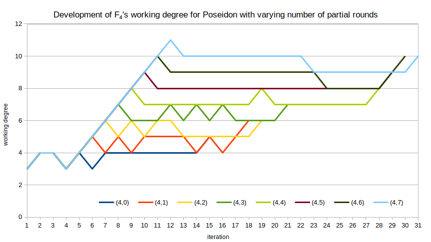
F4’s working degree
The working degree of F4 is quite “bouncy” for the polynomial systems derived from Poseidon. For example, for $r_\text{full} = 4$ with varying number of partial rounds, we can plot the working degree of F4 against the iteration that degree occurred in. While the overall tendency is “up,” there are many iterations for which the working degree does not change, or even drops. I am unsure what exactly this means in terms of security, or if it means anything at all.
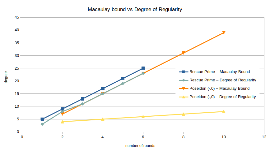
Comparison between Rescue-Prime and Poseidon
One of the most notable differences between the polynomial systems for Rescue-Prime and Poseidon is the growth rate of their respective degrees of regularity. For example, consider the following plot, where I have repeated the data for Rescue-Prime from above and added the Macaulay bound and degree of regularity for (·,0)-Poseidon, i.e., varying the number of full rounds.
While the Macaulay bounds are almost identical, the observed degrees of regularity differ greatly.
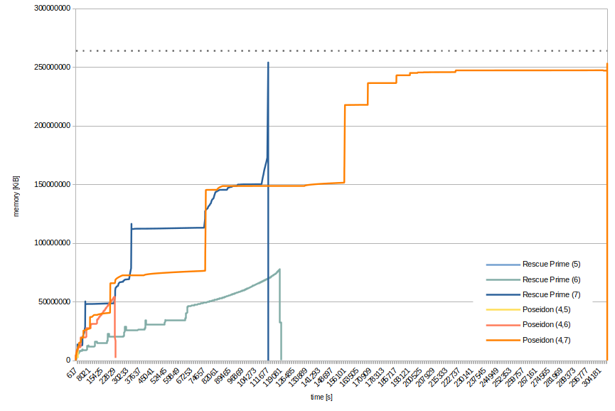
It’s also nice to see the development of the used memory for a few instances, even though that comparison is not very important. Below figure shows the required memory over time for 5, 6, and 7-round Rescue-Prime and (4,5), (4,6), (4,7)-round Poseidon. The respective smallest of these Recall that 7-round Rescue-Prime and (4,7)-round Poseidon both ran out of memory, i.e., terminated abnormally.
By the jumps in memory consumption you can pretty clearly see where a new, bigger matrix was constructed. This corresponds to the iterations of F4. Exponential – or binomial – growth being what it is, it does not make sense to plot instances with less rounds. Already, 5-round Rescue-Prime and (4,5)-round Poseidon are barely visible in the lower-left corner of the figure. The dotted line corresponds to the total available memory.
Conclusion
The data suggests that the implicit assumption about the regularity of the polynomial system arising from Poseidon is wrong: the difference between the Macaulay bound and the observed degree of regularity implies that the system is irregular. This has direct consequences for the minimum number of rounds required to achieve a target security level. For example, for $p = 65519$ and state size $2$, we recommend $(8,24)$ rounds as opposed to $(8,9)$ rounds.
An interesting open question is how to interpret the “bounciness” of F4‘s working degree when computing a Gröbner basis for a Poseidon-derived system. The significance of this behavior is completely unclear.
Another open question regards the discrepancy in the observed growth of the degree of regularity for Rescue and Rescue-Prime. Regardless, the data supports the security argument of Rescue-Prime: adding one half round at either end, i.e., transforming “plain” Rescue into Rescue-Prime, does not seem to decrease security.
All things told, no successful Gröbner basis attack could be performed for anything approaching realistic round numbers – even for this tiny Sponge construction.
References
Aly, A., Ashur, T., Ben-Sasson, E., Dhooghe, S., Szepieniec, A.: Design of Symmetric Primitives for Advanced Cryptographic Protocols. IACR ToSC 2020(3), 1–45(2020)
J.-C. Faugère. FGb: A Library for Computing Gröbner Bases. In Komei Fukuda, Joris Hoeven, Michael Joswig, and Nobuki Takayama, editors, Mathematical Software ICMS 2010, volume 6327 of Lecture Notes in Computer Science, pages 84-87, Berlin, Heidelberg, September 2010. Springer Berlin / Heidelberg.
Grassi, L., Khovratovich, D., Rechberger, C., Roy, A., Schofnegger, M.: Poseidon: A New Hash Function for Zero-Knowledge Proof Systems. In: USENIX Security. USENIXAssociation (2020)
Szepieniec, A., Ashur, T., Dhooghe, S.: Rescue-Prime: a Standard Specification (SoK). Cryptology ePrint Archive, Report 2020/1143 (2020)
Appendix – Summary of Rescue-Prime and Poseidon
Below, I have put some figures summarizing the AOCs Rescue-Prime [4] and Poseidon [3], respectively. The input, output, and constants are all vectors of the same length. They are contracted here to simplify presentation.
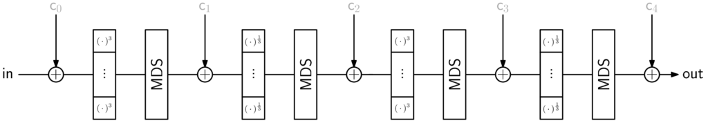
The first figure depicts $2$-round Rescue-Prime. Note that a single round, made up of two half rounds, first uses exponent $3$ and then $\frac{1}{3}$.
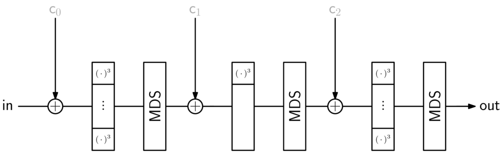
The second figure shows (2,1)-round Poseidon, i.e., the instance has 2 full rounds – 1 at the beginning, 1 at the end – and 1 partial round.
Appendix – Raw Data of the Experiments
Below, you can find the data this post is based on. Each experiment, say, (4,3)-Poseidon, comes with 4 files:
poseidon_65519_(4, 3)_fgb_debug.txt – debug information of FGb, described on page 12 in this document.
poseidon_65519_(4, 3)_mem.txt – memory requirements over time, in KiB, one row per second.
poseidon_65519_(4, 3)_summary.txt – includes time & memory measurements, degrees, data from FGb.
poseidon_65519_(4, 3)_sys.txt – the polynomial system for which the Gröbner basis was computed.
We have published an introductory paper [0] about Gröbner basis attacks on AOCs. Whether you’re looking for an intuitive way into the world of Gröbner basis computations, or want to look up a certain detail about the attack pipeline, or are simply curious to learn a few neat tricks and algorithms, it should be to your liking. A background in computer science probably helps when reading the document, but I encourage you to have a look in any case.
Broadly summarized, the paper
covers the basic definitions.
shows how solution readout works.
explains Buchberger’s algorithm, as well as F4 and F5.
describes the XL-family, especially Mutant XL.
goes into great detail about term-order change algorithm FGLM.
intuits the Gröbner Walk.
presents interesting and relevant open questions.
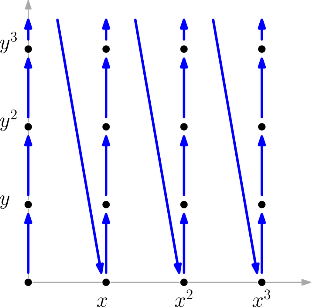
The document aims for intuition as opposed to complete rigor, but the many references make it easy to start digging deeper. A major plus: explaining things intuitively often means pictures! For example, did you know what a monomial order looks like when visualized? Below, you can see the orders lex and degrevlex in blue and red, respectively.
Or how about the Gröbner fan of a particular polynomial ideal? Admittedly, if you already know what a Gröbner fan is, you have probably seen pictures of some. But if you don’t yet know, maybe below illustration of a Gröbner Walk piques your curiosity to find out what it is all about.
No matter your motivation or background, I hope the SoK has something for you. And if you have any feedback, don’t hesitate to contact us!
When designing a symmetric cryptographic primitive, conventional wisdom has it that
the “simpler” an algebraic model of the primitive, the less secure, and
a primitive’s algebraic model becomes “complex” by mixing operations from different algebras, like finite fields, or vector spaces.
For example, take the Addition-Rotation-XOR (ARX) design principle. Adding two $n$-bit strings modulo $2^n$ is one of the simplest possible operations for a computer. However, for Gröbner basis analysis of the primitive, we need a polynomial $f^+$ modeling the same operation, and the polynomial’s coefficients need to come from a field. Unfortunately, the field-native addition of two elements from $\mathbb{F}_{2^n}$ corresponds to XOR. Representing addition of bit strings modulo $2^n$ requires a polynomial of quite high degree. That’s bad for algebraic cryptanalysis.
Another consequence is that ARX primitives are no suitable candidates when low arithmetic complexity is required, which includes most modern Zero-Knowledge Proof Systems. This is one of the reasons why hash functions like Rescue Prime [1,3] and Poseidon [2] have emerged: simple algebraic representability. Roughly summarized, they’re designed to have polynomial representation simple enough – meaning few and low-degree polynomials – for efficient use in Zero-Knowledge Proof Systems, but complex enough to thwart the most efficient algebraic analysis methods. Most notably, all operations can be easily modeled over the same finite field, counter to the second piece of “conventional wisdom” above.
Reinforced Concrete’s Subfunction “Bars”
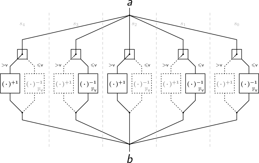
The recently proposed Plookup-friendly Hash function “Reinforced Concrete” [4] can be seen as a mix of those two paradigms: all subfunctions are either linear or can be expressed as low-degree polynomials over some finite field, but not always over the same field. The algebraically most interesting subfunction, “Bars,” is the primary defense against Gröbner basis attacks. It essentially consists of the following steps:
Variable-base decomposition of the input
Conditional application of a small S-Box
Variable-base composition
Visualization of Reinforced Concrete’s subfunction “Bars”
Variable-base decomposition Decomposition takes a field element and returns a tuple. Giving intuition with an example, take a = 318. Fix-base decomposing a with base 10, we can write $\boldsymbol{\textsf{a}} = 3\cdot(10\cdot 10) + 1\cdot(10) + 8$, and decomposition thus results in $(3, 1, 8)$. Choosing a variable base instead, say $(s_2, s_1, s_0) = (13, 9, 12)$, we can write $\boldsymbol{\textsf{a}} = 2\cdot(9\cdot 12) + 8\cdot(12) + 6$, and this variable-base decomposition thus results in $(2, 8, 6)$. More formally, given base $(s_{n-1}, \dots, s_0)$, we can decompose like this: $$\begin{align*}a_0 &= \boldsymbol{\textsf{a}}\bmod{s_0},\\a_i &= \frac{\boldsymbol{\textsf{a}}-\sum_{j<i}a_j\prod_{k<j}s_k}{\prod_{j<i}s_j}\bmod{s_i}.\end{align*}$$
Conditional S-Box application A permutation is applied to each $a_i$ that is smaller or equal to a threshold value $\textsf{v}$. For the Reinforced Concrete instance this post is concerned with, $\textsf{v}$ is prime, and the permutation amounts to inversion of $s_i$ as an element of finite field $\mathbb{F}_\textsf{v}$. Picking up the example from above, let $\textsf{v} = 7$ and $(a_2, a_1, a_0) = (2, 8, 6)$. The S-Box is applied to $a_2$ and $a_0$, but not to $a_1$, because it is greater than $\textsf{v}$. The multiplicative inverse of $2$ in $\mathbb{F}_7$ is $4$, that of $6$ is $6$. The result is $(b_2, b_1, b_0) = (4, 8, 6)$. A more formal description of this step is $$b_i=\textsf{S-Box}(a_i) = \begin{cases}a_i &\text{ if } a_i > \textsf{v},\\\textsf{inv}_{\mathbb{F}_\textsf{v}}(a_i) &\text{ if } a_i \leqslant \textsf{v}.\end{cases}$$
Variable-base composition Going back from a tuple of elements to one field element, composition is the inverse of the first step. Finishing up the running example, composition gives $\boldsymbol{\textsf{b}} = 4\cdot(9\cdot 12) + 8\cdot(12) + 6 = 534$. Formally, we have $$\boldsymbol{\textsf{b}} = \sum_i b_i \prod_{j<i} s_j.$$
A Polynomial System for “Bars”
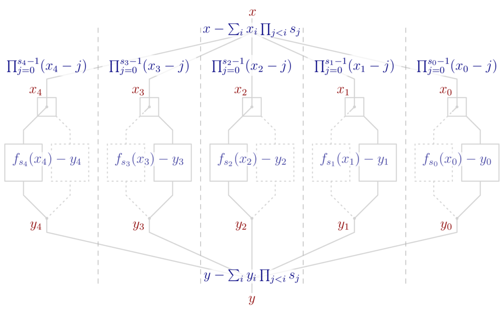
Building a polynomial model for Bars is most straightforwardly done by modeling each of the steps. Let’s start with the decomposition of input $x$, where $x$ is a variable. We introduce one new variable for each decomposition-basis element $s_i$. Decomposition can then be written as $x -\! \sum_i x_i \prod_{j<i}s_j$, which is a linear polynomial. However, this polynomial does not guarantee that $x_i$ can only take values in the range $[0, s_i[$. We therefore need to add additional polynomial constraints that can only be satisfied if $x_i$ is in the specified range. The polynomial we’re looking for is $\prod_{j=0}^{s_i-1}(x_i – j)$: it is zero if and only if $0 \leqslant x_i < s_i$. Summarizing, we introduce $n$ polynomials, one of degree $s_i$ for each element in the decomposition’s variable base.
For composition, we introduce another $n$ many variables $y_i$ for the output of the S-Boxes, and variable $y$ for the output of Bars. Then, composition can be written as $y -\! \sum_i y_i \prod_{j < i} s_j$, much like before. The condition $0 \leqslant y_i \leqslant s_i$ will be implicitly ensured by the next and last step.
All that remains is linking the $x_i$ with the $y_i$ by modeling the conditional application of the S-Box. I have tried cleverly applying the Bézout identity, but the resulting polynomials were of considerably higher degree than just bluntly applying Lagrange interpolation. As a result, getting the polynomials for this step is easy but not pretty: create a list with $s_i$ many entries $(i, \textsf{S-Box}(i))$ and univariably interpolate this list using variable $x_i$, resulting in polynomial $f_{s_i}(x_i)$. Then, $f_{s_i}(x_i) – y_i$ correctly relates variables $x_i$ and $y_i$. In total, this means adding another $n$ polynomials of degrees $s_i – 1$, respectively.
The variables (red) and polynomials (blue) modeling Bars
Computing the Gröbner Basis
Summarizing the polynomial system, we have introduced $2n+2$ variables, as well as $2n+2$ polynomials. Two of these polynomials – composition and decomposition – are linear, and for each $s_i$, we have one polynomial of degree $s_i$ and one of degree $s_i – 1$.
Assuming this polynomial system is a regular sequence – and my experiments indicate this to be the case – the Macaulay bound helps with upper bounding the complexity of the Gröbner basis computation. For a set of polynomials $\{f_0, \dots, f_{m-1}\}$, the Macaulay bound is $$1 + \sum_i \deg(f_i) – 1.$$ Plugging in the numbers of the just built polynomial system modeling subfunction Bars, the Macaulay bound is $1 + \sum_i s_i – 1 + \sum_i s_i – 2 = 1 – 3n + 2\sum_i s_i$. The suggested parameters for the BN254 curve are $n=27$ and each of the $s_i$ lies in the range $[668, 703]$. This means the Macaulay bound is enormous: $37408$ to be exact.
Computing the Gröbner basis for a regular sequence that has a big Macaulay bound is, generally speaking, very hard. Unfortunately, we currently only have worst-case bounds, but no way to (tightly) estimate the complexity of computing the Gröbner basis for a concrete polynomial system. Instead, we perform tests on toy examples and see if everything holds up.
Let’s build the polynomial system for Bars based on some toy-sized parameters: $p=47$, $v=5$, $n=2$, and $s_0=s_1=7$. We’ll have to deal with $6$ variables and $6$ equations, and the Macaulay bound for the resulting system is $23$. This is not nothing, but it’s also not very big: the polynomial system of 6 full rounds of Poseidon (with state size 2) has the same Macaulay bound, and the system for 5 rounds of Rescue (also state size 2) has comparable Macaulay bound $21$. For reference, I’ve put the resulting polynomial system $\mathcal{F}^{[7,7]}_{(47,5)}$ below, but reading it is not necessary for the rest of this post.
Computing the associated Gröbner basis (in degrevlex order) is surprisingly fast, and the degree of the highest degree polynomial appearing in any intermediary step is $7$. That’s not even close to the Macaulay bound! So why is the computation so much easier than anticipated? There are some further observations to be made, for which we first need to go on a slight tangent.
Vectors of Origin
For polynomial sequence $\mathcal{F} = (f_0, \dots, f_{m-1})$, any element $g$ from its Gröbner basis is a (non-linear) combination of the input elements: $g = \sum_i h_i\cdot f_i$ or, using vector notation, $g = \boldsymbol{h}\cdot\mathcal{F}$. I call $\boldsymbol{h}$ the vector of origin for $g$ because it tells us where $g$ originates from in relation to $\mathcal{F}$. The set of vectors of origin describing the entire Gröbner basis is packed with information, and not all of it is easy to interpret. But something that’s glaringly obvious in any vector of origin is a zero-entry. A zero in position $i$ in vector of origin $\boldsymbol{h}$ means that $f_i$ was unnecessary for computing $g$.
I’ve used the tool VooDoo to compute the vectors of origin for the polynomial system $\mathcal{F}^{[7,7]}_{(47,5)}$. For clarity of reading, any big polynomial is replaced by $\bullet$. Here’s what the vectors look like:
See the pattern? It appears that computing the Gröbner basis for $\mathcal{F}^{[7,7]}_{(47,5)}$ can be reduced to computing on multiple smaller systems. After all, the polynomials describing one S-Box are pretty much completely independent from the polynomials describing another S-Box. Dividing and conquering is a strategy that is usually impossible for computing a Gröbner basis, but in this specific case, it’s back on the table: the Macaulay bound for the sub-system describing one S-Box is $1+ s_i – 1 + s_i – 2$, amounting to $12$ in our toy example. This doesn’t fully explain the discrepancy to the observed highest degree of $7$ yet, suggesting that more interesting riddles are waiting to be solved.
Above analysis doesn’t mean that using subfunction Bars is unsuitable for preventing Gröbner basis attacks. However, looking at the entire polynomial system and relying on the complexity upper bound for the Gröbner basis computation implied by the Macaulay bound is probably too optimistic.
References
Aly, A., Ashur, T., Ben-Sasson, E., Dhooghe, S., Szepieniec, A.: Design of Symmetric Primitives for Advanced Cryptographic Protocols. IACR ToSC 2020(3), 1–45(2020)
Grassi, L., Khovratovich, D., Rechberger, C., Roy, A., Schofnegger, M.: Poseidon: A New Hash Function for Zero-Knowledge Proof Systems. In: USENIX Security. USENIX Association (2020)
Szepieniec, A., Ashur, T., Dhooghe, S.: Rescue-Prime: a standard specification (SoK). Cryptology ePrint Archive, Report 2020/1143 (2020), https://eprint.iacr. org/2020/1143
Barbara, M., Grass, L., Khovratovich, D., Lueftenegger, R., Rechberger, C., Schofnegger, M., Walch, R.: Reinforced Concrete: Fast Hash Function for Zero Knowledge Proofs and Verifiable Computation. Cryptology ePrint Archive, Report 2021/1038 (2021), https://eprint.iacr.org/2021/1038
Appendix: The Polynomial System
Below, you can find the polynomial system for the toy-sized parameters from above. Note how the polynomials corresponding to the S-Boxes are identical, which is due to $s_0 = s_1$ and does not generally hold. The same is true for the polynomials ensuring $0 \leqslant x_i < s_i$. However, the similarities between the decomposition polynomial and the composition polynomial is inherent.
When attacking an AOCs using Gröbner bases, the most relevant question is: how complex is the Gröbner basis computation? One commonly used estimation is based on the degree of regularity. Intuitively, the degree of regularity is the degree of the highest-degree polynomials to appear during the Gröbner basis computation. (Whether this metric is good for estimating the AOC’s security is a different matter.)
Unfortunately, different authors define the term “degree of regularity” differently. In this post, I use the understanding of Bardet et al. [1,2], which coincides with the well-defined Hilbert regularity.
I first introduce the required concepts, and then make them more tangible with some examples. Lastly, there is some code with which the Hilbert regularity can be computed.
Definition of the Hilbert Regularity
Let $\mathbb{F}$ be some field, $R = \mathbb{F}[x_0, \dots, x_{n-1}]$ a polynomial ring in $n$ variables over $\mathbb{F}$, and $I \subseteq R$ a polynomial ideal of $R$.
The affine Hilbert function of quotient ring $R/I$ is defined as $${}^a\textsf{HF}_{R/I}(s) = \dim_\mathbb{F}\!\left(R_{\leqslant s} \middle/ I_{\leqslant s}\right).$$ For some large enough value $s_0$, the Hilbert function of all $s \geqslant s_0$ can be expressed as a polynomial in $s$.1 This polynomial, denoted ${}^a\textsf{HP}_{R/I}(s)$, is called Hilbert polynomial. By definition, the values of the Hilbert function and the Hilbert polynomial coincide for values greater than $s_0$.
The Hilbert regularity is the smallest $s_0$ such that for all $s \geqslant s_0$, the evaluation of the Hilbert function in $s$ equals the evaluation of the Hilbert polynomial in $s$.
By the rank-nullity theorem, we can equivalently write the Hilbert function as $${}^a\textsf{HF}_{R/I}(s) = \dim_\mathbb{F}\! \left( R_{\leqslant s} \right) – \dim_\mathbb{F}\! \left( I_{\leqslant s}\right).$$ This is a little bit easier to handle, because we can look at $R$ and $I$ separately and can ignore the quotient ring $R/I$ for the moment. By augmenting $R$ with a graded monomial order, like degrevlex, we can go one step further and look at leading monomials $\textsf{lm}$ only: the set $\{ \textsf{lm}(f) \mid f \in I, \deg(f) \leqslant s \}$ is a basis for $I_{\leqslant s}$ as an $\mathbb{F}$-vector space.2 Meaning we don’t even need to look at $I$, but can restrict ourselves to the ideal of leading monomials $\langle \textsf{lm}(I) \rangle$. $${}^a\textsf{HF}_{R/I}(s) = \dim_\mathbb{F}\!\left(R_{\leqslant s}\right) – \dim_\mathbb{F}\!\left( \langle \textsf{lm}(I) \rangle_{\leqslant s}\right).$$
One way to get a good grip on $\langle I \rangle$ is through reduced Gröbner bases. A Gröbner basis $G$ for ideal $I$ is a finite set of polynomials with the property $\langle G \rangle = \langle I \rangle$ and, more relevant right now, $\langle \textsf{lm}(G) \rangle = \langle \textsf{lm}(I) \rangle$. This means it’s sufficient to look at (the right combinations) of elements of $\textsf{lm}(G)$, which is more manageable.
Example: 0-Dimensional Ideal
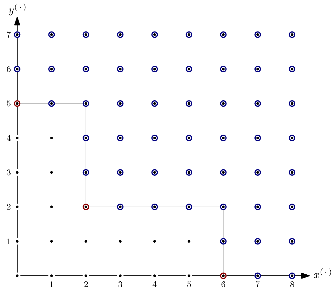
Let’s start with a super simple polynomial system: $$G = \{x^6, x^2y^2, y^5\} \subseteq \mathbb{F}[x,y], \quad I = \langle G \rangle$$ for some finite field $\mathbb{F}$. This is a zero-dimensional, monomial (thus homogeneous) ideal. That’s about as special as a special case can get. Note that here, we have $I = \langle \textsf{lm}(I) \rangle$, but this doesn’t generally hold. Dealing with a super-special case also means that the Hilbert polynomial is relatively boring, but that’s fine for starting out. $G$ is the reduced Gröbner basis for $I$, and we’ll use its elements to help computing the Hilbert function.
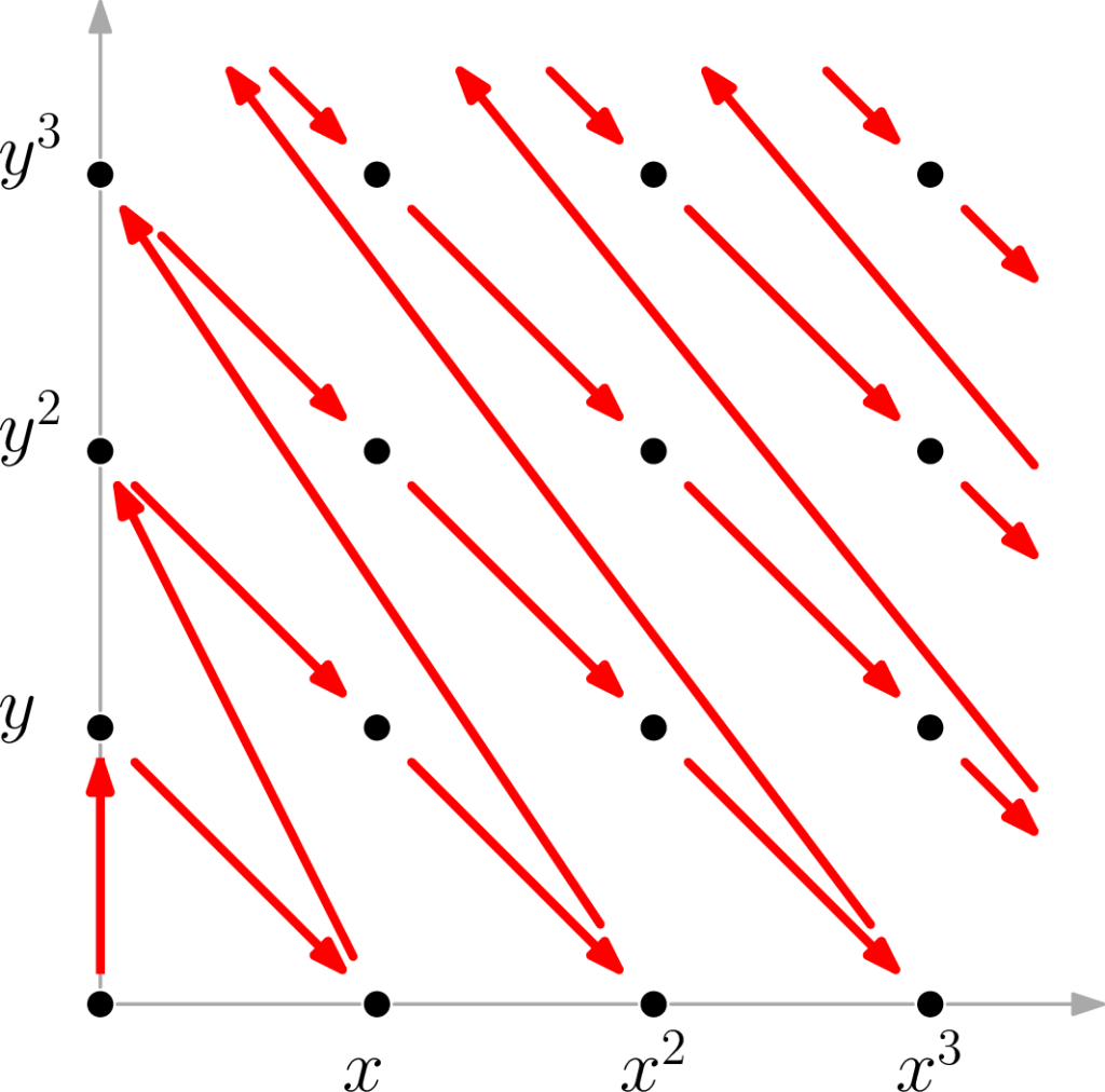
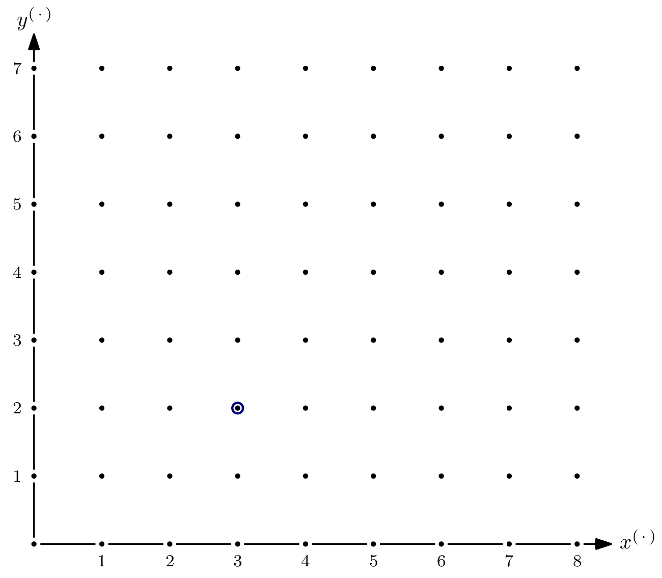
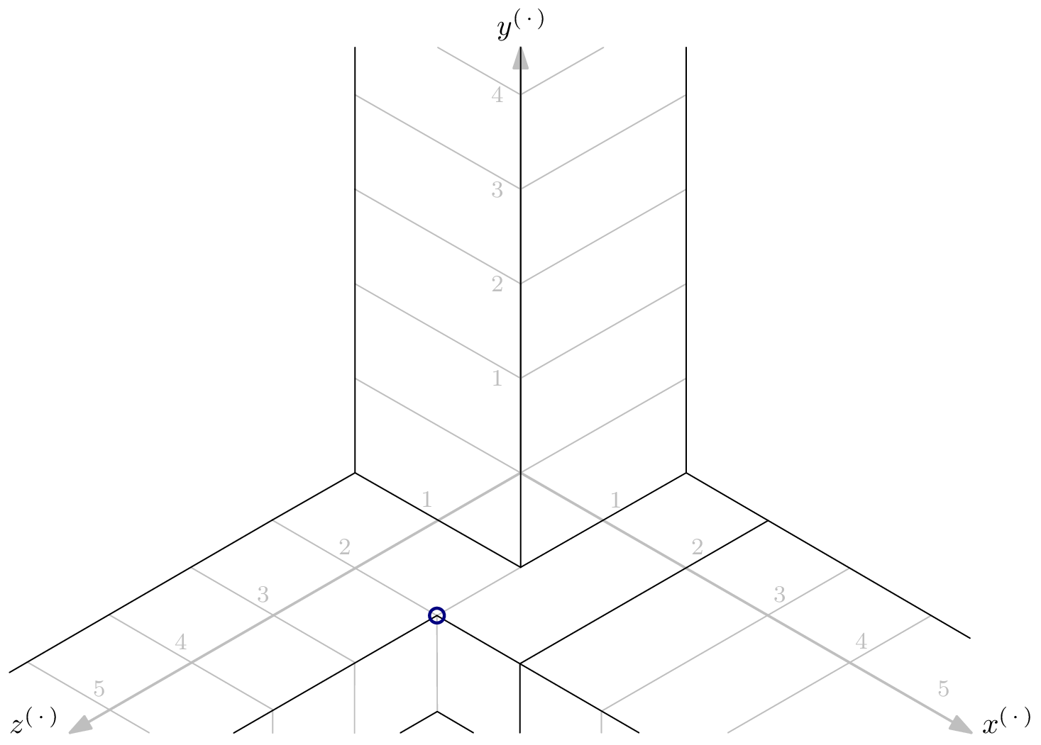
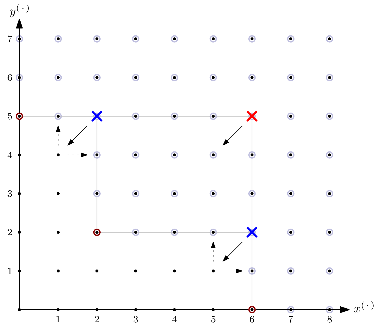
A benefit of ideals in two variables is: we can draw pictures.
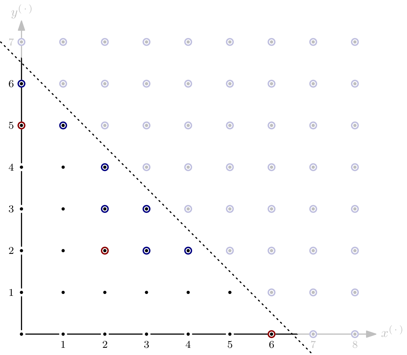
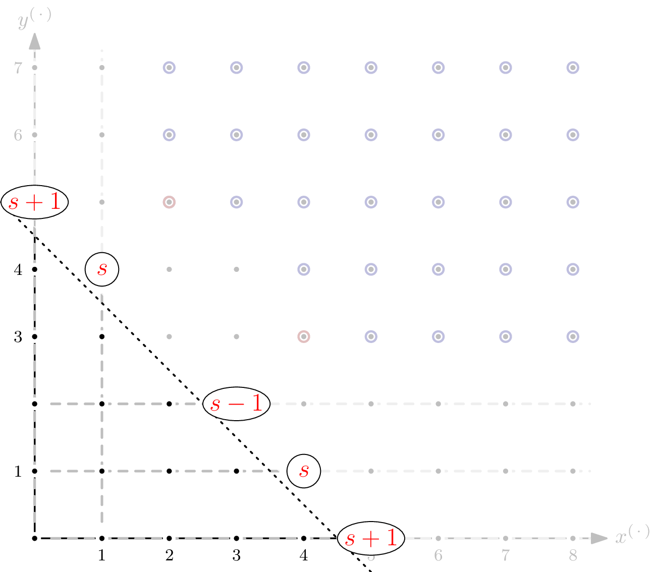
This is what the monomials of $\mathbb{F}[x,y]$ as an $\mathbb{F}$-vector space look like. Well, at least the part $\{x^ay^b \mid a \leqslant 8, b \leqslant 7 \}$. After all, $\mathbb{F}[x,y]$ as an $\mathbb{F}$-vector space has infinite dimension. I have (arbitrarily) highlighted $x^3y^2$, i.e., coordinate $(3,2)$, to give a better understanding of what the picture means.
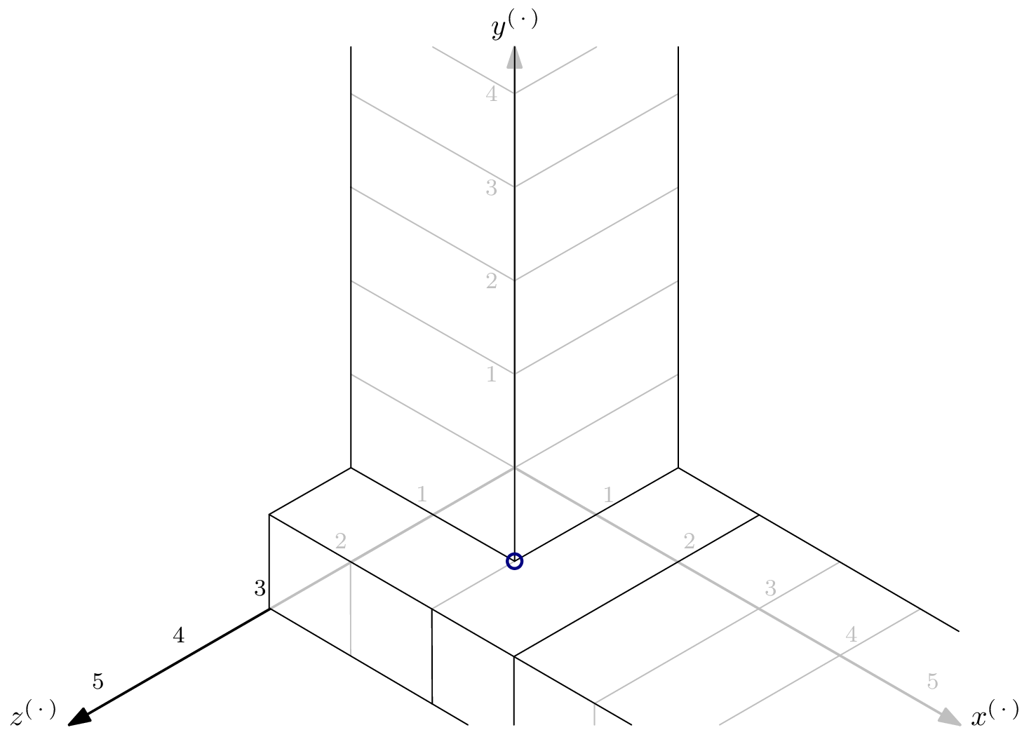
Since $I$ is a monomial ideal, we can highlight every element in $I$. The circles of the elements of the Gröbner basis $G$ are red. The zig-zig pattern of the boundary between $x^ay^b \in I$ and $x^ay^b \notin I$ is inherent, and generalizes to higher dimensions, i.e., more variables. Because of the zig-zagging, the set of monomials not in $\langle \textsf{lm}(I) \rangle$ is referred to as staircase of $I$.
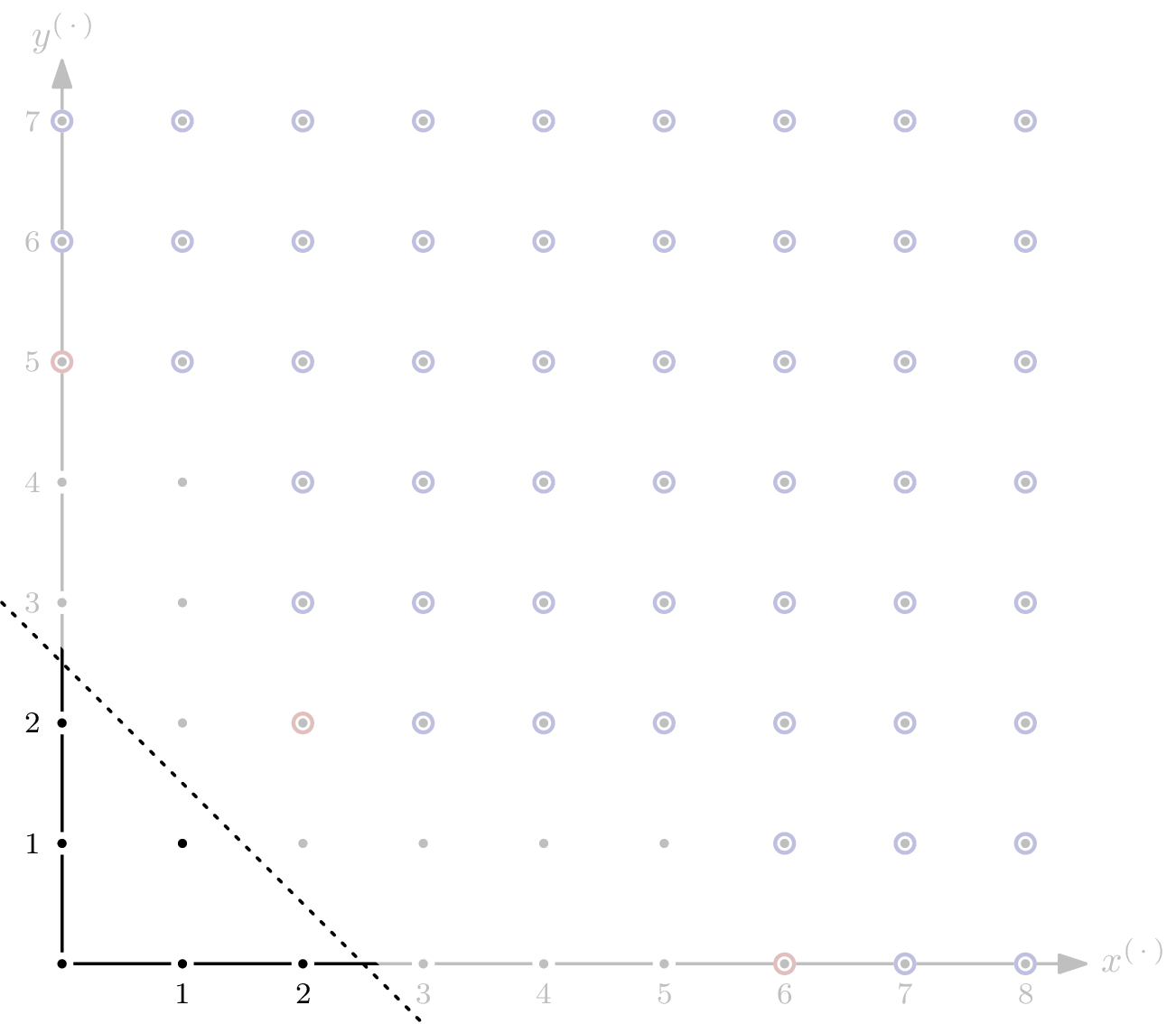
Let’s start computing the Hilbert function for $R/I$. The $\mathbb{F}$-vector space dimensions of $R_{\leqslant s}$ and $I_{\leqslant s}$ are simply the number of monomials in $R$ respectively $I$ with degree $\leqslant s$. Getting those numbers is easy – it amounts to counting dots in the picture! For example, for $s=2$, we have ${}^a\textsf{HF}_{R/I}(2)=5-0=5$:
No monomial of total degree less than or equal to 2 is in $I$, so computing the Hilbert function is a little bit boring here.
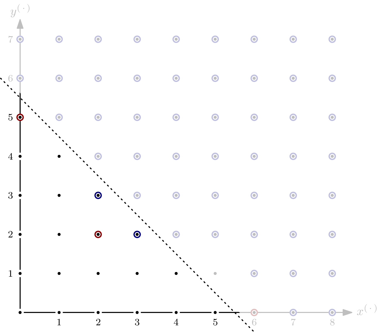
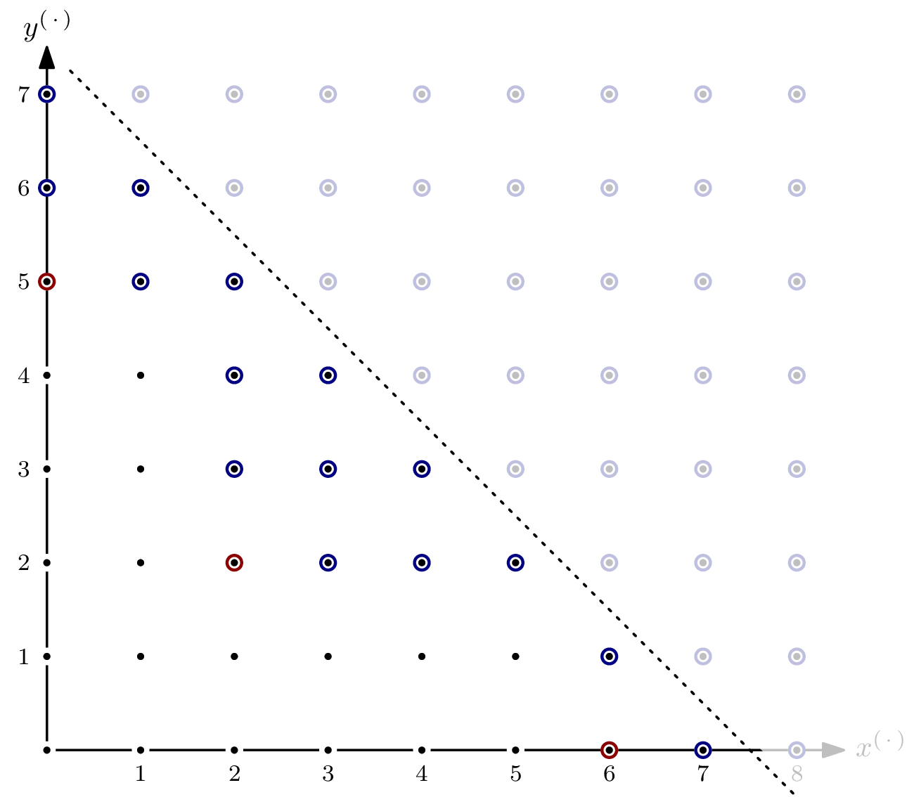
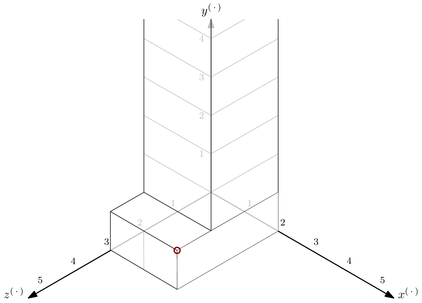
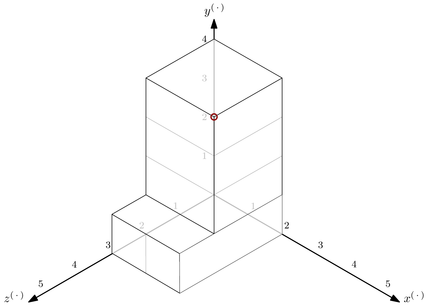
The value of the Hilbert function ${}^a\textsf{HF}_{R/I}(5)$ is more interesting: Some monomials of degree $\leqslant 5$ are indeed elements of $I$, and thus $\dim I_{\leqslant 5}$ is not $0$ but $4$. In particular, we have ${}^a\textsf{HF}_{R/I}(5)=21 – 4=17$. For $s=6$, we have ${}^a\textsf{HF}_{R/I}(6)=28-10=18$:
From this point forward, increasing $s$ will not change the value of the Hilbert function – the dimension of $I_{\leqslant s}$ as an $\mathbb{F}$-vector space grows with the same rate as the dimension of $R_{\leqslant s}$, since all monomials not in $I$ are of lesser total degree. Expressed differently, all monomials above the line are elements of both $I$ and $R$ – the values of the Hilbert function doesn’t change by increasing $s$.
From this, two things follow:
The Hilbert polynomial of $R/I$ is the constant $18$. (That’s why I said it’s relatively boring. A more interesting case follows.)
The Hilbert regularity of $R/I$ is $6$, since ${}^a\textsf{HF}_{R/I}(s) = {}^a\textsf{HP}_{R/I}(s)$ for all $s \geqslant 6$.
Example: Ideal of Positive Dimension
As hinted at above, whether or not $I$ is a monomial ideal does not matter for computing the Hilbert function or the Hilbert polynomial, because $\textsf{lm}(I)$ behaves exactly the same. What does matter, though, is the dimension of $I$. In the previous example, $I$ was of dimension 0, and the Hilbert polynomial of $R/I$ was a constant. That’s not a coincidence.
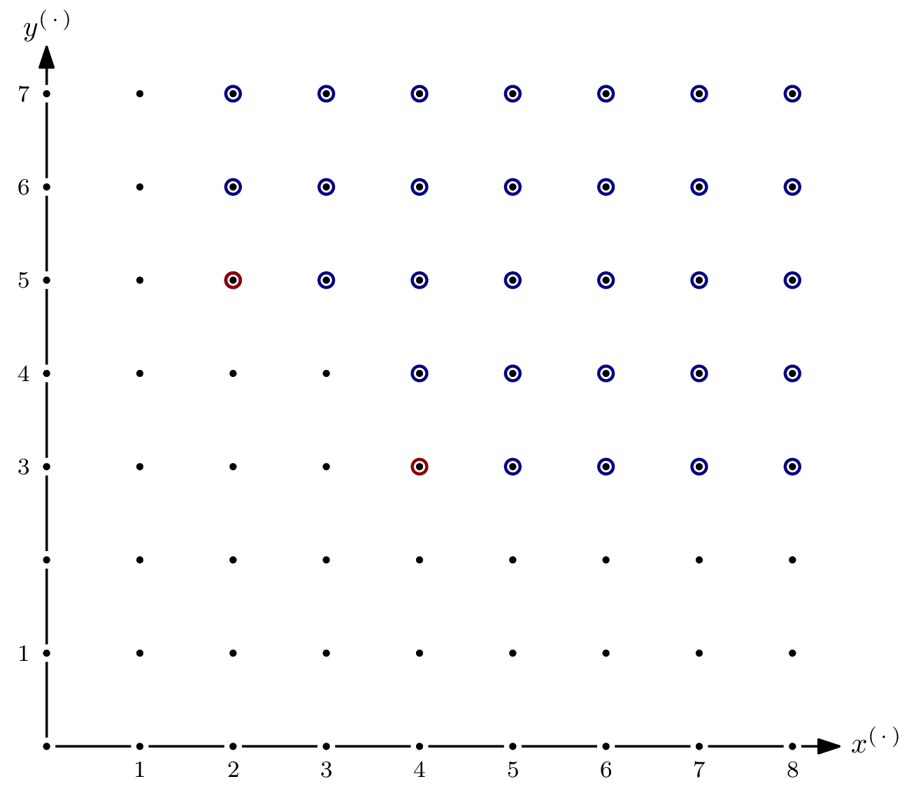
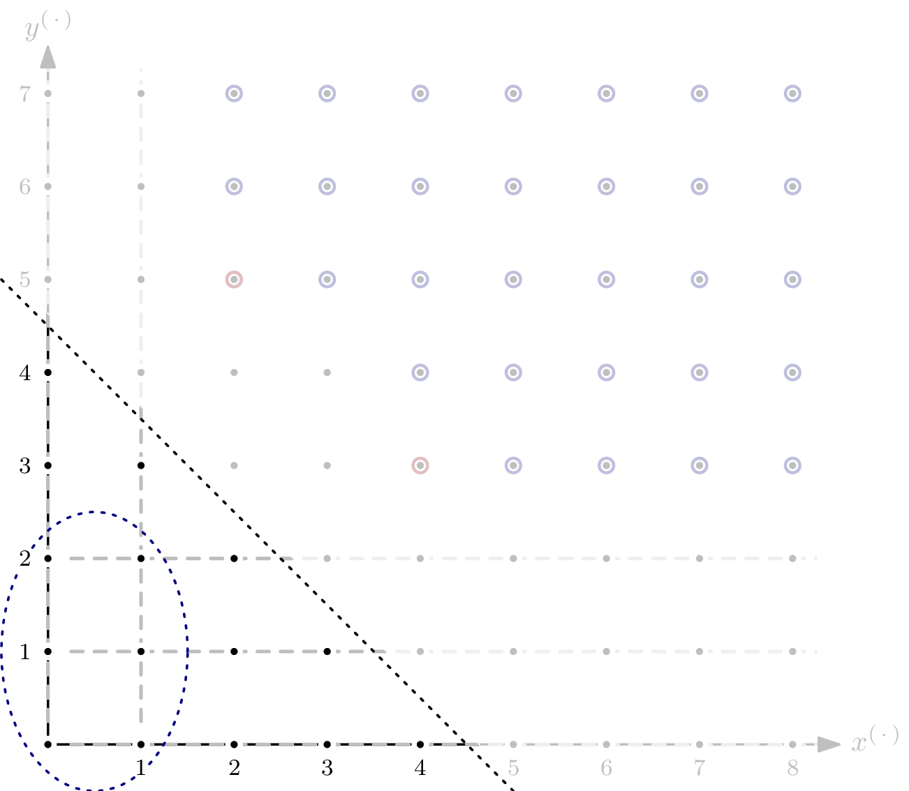
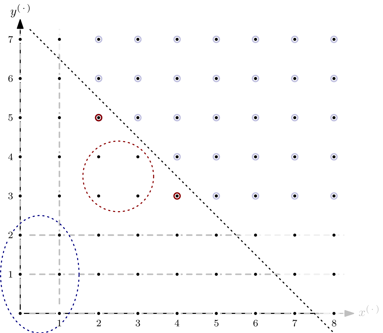
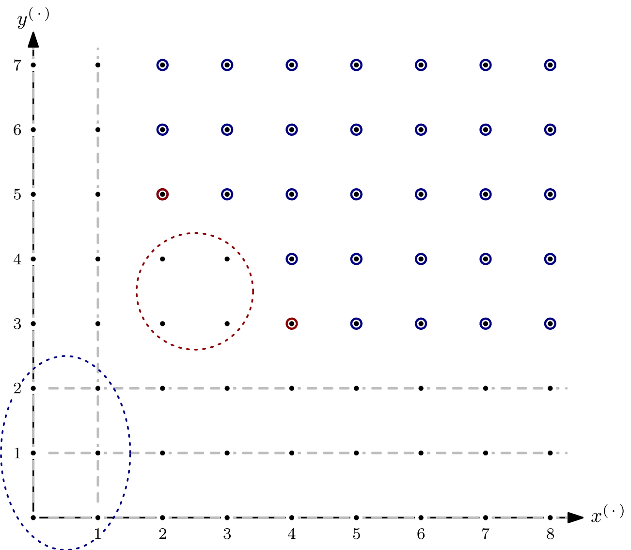
Even though the ideal spanned by the polynomial system modelling an AOC will usually be zero-dimensional, it’s interesting to see what happens if it isn’t. Let’s take $G = \{x^4y^3, x^2y^5\} \subseteq \mathbb{F}[x,y]$ and $I = \langle G \rangle$.
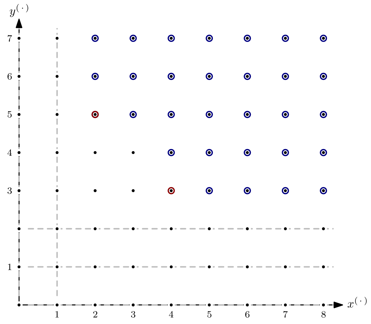
As you can see, there are parts of the staircase that extend to infinity. That’s a direct consequence of $I$ having positive dimension, or, equivalently, variety $V(I)$ not having finitely many solutions. In the picture below, I’ve indicated the staircase’s five subspaces of dimension $1$ by dashed, gray lines.
For the Hilbert function, only monomials in $I$ of degree $\leqslant s$ are relevant. For each of the five subspaces, we can express the matching number of elements as a polynomial in $s$.
The sum of these five polynomials is $5s+1$, which corresponds to the total number of monomials in the staircase of $I$ of degree $\leqslant s$ that lie in the staircase’s $1$-dimensional subspaces – except that some elements are counted more than once. Since the intersection of two orthogonal $1$-dimensional subspaces is of dimension $0$, we can simply add a constant correction term.3
Adding the correction term of $-6$ gives $5s-5$ as a (preliminary) Hilbert polynomial for $I$. We’re not completely done yet: for $s > 4$, there are monomials not in $I$ that are also not in any of the $1$-dimensional subspaces – for example $x^3y^3$. Of those, we only have finitely many. In the example, it’s $4$.
After adding the second correction term, we have ${}^a\textsf{HP}_{I/R}(s)=5s-1$.
By finding the Hilbert polynomial, we also computed the Hilbert regularity of $R/I$: it’s $7$. In other words, for $s\geqslant 7$, we have $\dim_\mathbb{F}(R/I) = {}^a\textsf{HF}_{R/I}(s) = {}^a\textsf{HP}_{R/I}(s) = 5s-1$.
This coincides with the distance of the closest diagonal4 such that all “overlapping” as well as all $0$-dimensional parts of the staircase are enclosed – the red and blue dashed circles, respectively, in above picture.
More Variables, More Dimensions
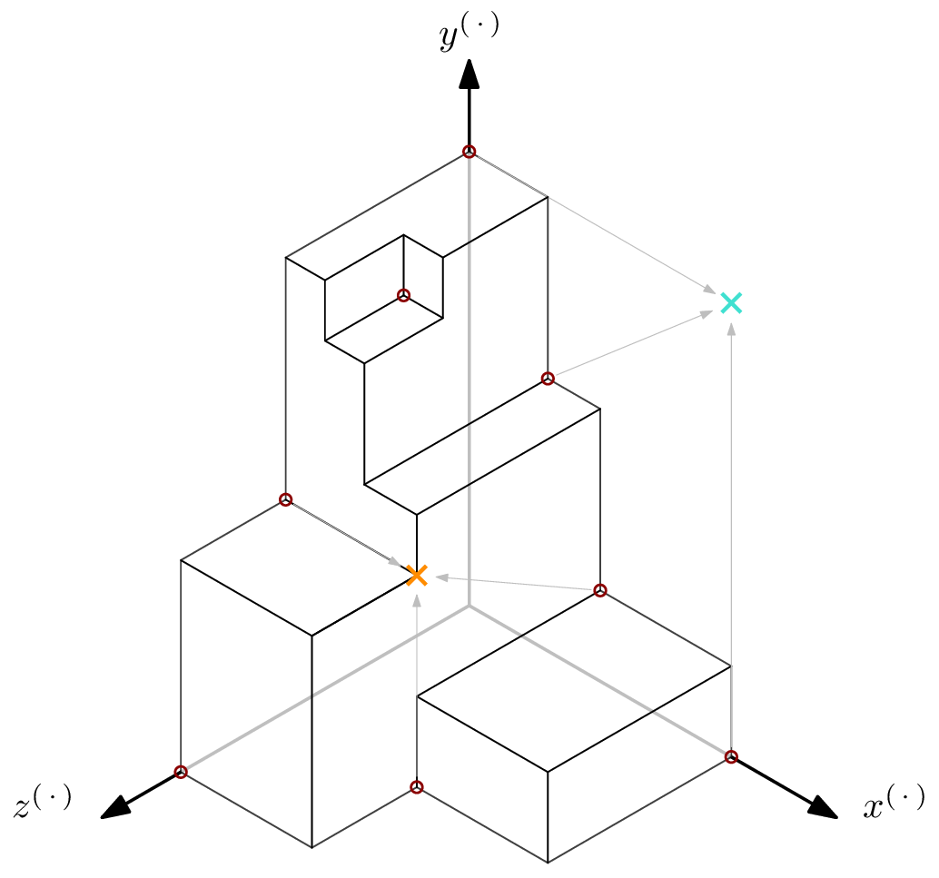
The intuition of the two-dimensional examples above translate to higher dimensions: find the most distant corner of the blue circle – the parts where positive-dimensional subspaces of the variety overlap – and the red circle – the variety’s part of dimension zero – and take the distance of the farther of these two corners as the Hilbert regularity. However, finding the corners becomes less trivial. Let me demonstrate with a staircase consisting of three “tunnels” that we’ll successively modify.
Above staircase is defined by $G=\{x^2y, x^2z^3, yz^2\}$. No monomials exist in the red bubble – every point is part of a subspace of dimension $1$. The blue corner is the monomial defining the enclosing space of the parts where positive-dimensional subspaces overlap. It coincides with the least common multiple (lcm) of the three elements of $G$, namely $m=x^2yz^3$. The Hilbert regularity can be read off from $m$: the hyperplane’s required distance is $\deg(x^{(2-1)}y^{(1-1)}z^{(3-1)})=4$.
That was easy enough. Let’s take a look at $G’ = \{x^2y, yz^2, z^3\}$. The staircase looks similar, with the exception for the “$z$-tunnel.”
Even though $m$ from above is still on the “border” of $\langle G’ \rangle$, just as it was for $\langle G \rangle$, it no longer defines the enclosing space we’re looking for. Note that the lcm of the elements in $G’$ is still $m$, but the Hilbert regularity is now defined by the lcm of only two elements, $x^2y$ and $yz^2$, giving $m’ = x^2yz^2$. The Hilbert regularity has changed to $3$.
Let’s modify the staircase a little bit more, and look at $G^\dagger = \{x^2, yz^2, z^3\}$.
The Hilbert regularity can once again be found by looking at $m = x^2yz^3$, but the reason has changed. This time around, $m$ is the most distant corner of the volume enclosing all monomials not appearing in positive-dimensional subspaces of the variety – that’s the red bubble from before. And since only one “tunnel” remains, there’s no more overlap in positive-dimensional subspaces – the blue bubble, and with it the blue dot, have disappeared. Note that $m$ is once again the lcm of the three elements of $G^\dagger$.
For completeness sake, let’s close off the last of the tunnels by adding $y^4$ to $G^\dagger$. Monomial $m^\dagger = x^2y^4z^2$, being the lcm of $x^2$, $yz^2$, and $y^4$, is the Hilbert regularity-defining corner.
Computing the Regularity in sagemath
After having understood the Hilbert regularity, it’s time to throw some sagemath at the problem. Below, you can find two approaches. The first uses the staircase, like in the examples above. The second is based on the Hilbert series, which is explained further below.
The nice-to-visualize geometric approach
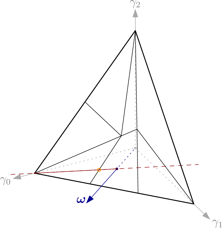
Using the geometric intuitions from above, we can compute the Hilbert regularity by finding all of the staircase’s corners. The code below only works for ideals of dimension 05 since the polynomial models I do research on are always of that kind.
The code computes all lcm’s of subsets of size $n$ of the Gröbner basis’ leading monomials, which we have determined as the points of interest above. Any such lcm corresponding to a monomial that’s flush to one of the $0$-planes is ignored as being degenerate – for example, the turquoise cross in below picture. Next, we check if the lcm-monomial is actually a corner of the staircase, by moving one step towards the origin along all axes. If the resulting monomial is in the ideal, it is not in the staircase, and thus not a corner – for example, the red cross in above picture. If, from the moved-to monomial, moving one step along any axis crosses the border of the staircase, we found a corner – for example, both of the blue crosses in above picture, but not the orange cross in the picture below. The distance of the furthest such corner corresponds to the Hilbert regularity.
With those pictures in mind, following the code should be fairly doable:
from itertools import combinations
def hilbert_regularity_staircase(I):
    '''
    Compute the Hilbert regularity of R/I where R = I.ring() and I.dimension() <= 0.
    This is done by iterating through all n-tuples of the Gröbner basis' leading monomials,
    computing their lcm, then determining if that lcm is actually a corner of the staircase.
    The corner that is the furthest from the origin determines the Hilbert regularity.
    '''
    if I.dimension() > 0:
        raise NotImplementedError(f"Ideal must not be of positive dimension, but has dim {I.dimension()}.")
    gens = I.ring().gens() # all variables
    n = len(gens)
    xyz = reduce(operator.mul, gens, 1)
    gb_lm = [f.lm() for f in I.groebner_basis()]
    I_lm = Ideal(gb_lm)
    hil_reg = 0
    for lms in combinations(gb_lm, n):
        m = lcm(lms)
        # are we considering a meaningful combination of lm's?
        # i.e., does every variable make an appearance in m?
        if len(m.degrees()) != n or not all(m.degrees()):
            continue
        m = m / xyz # 1 step towards origin along all axes
        assert I.ring()(m) == m.numerator() # no negative exponents, please
        m = I.ring()(m)
        # are we in a corner of the staircase?
        # i.e., not in the ideal, but moving 1 step along any axis, we end up in the ideal?
        if not m in I_lm and all([v*m in I_lm for v in gens]):
            hil_reg = max(hil_reg, m.degree())
    return hil_reg
The rigorous mathematical approach
The Hilbert regularity can also be computed using the Hilbert series. The Hilbert series is the formal power series of the (projective6) Hilbert function:$$\textsf{HS}_{R/I}(t) = \sum_{s=1}^{\infty}({}^a\textsf{HF}_{R/I}(s) – {}^a\textsf{HF}_{R/I}(s-1))t^s$$The Hilbert series’ coefficient of monomial $t^d$ is the number of monomials of degree $d$7 that are in $R$ but not in $I$. The Hilbert regularity coincides with the degree of the highest-degree consecutive term having positive coefficient.
For example, take $I$ from the very first example again, where we had $G = \{x^6, x^2y^2, y^5\}$. Evaluating the Hilbert function of $R/I$ gives $(1, 3, 6, 10, 14, 17, 18, 18, \dots)$. The Hilbert series of $R/I$ is $$\textsf{HS}_{R/I}(t) = 1 + 2t + 3t^2 + 4t^3 + 4t^4 + 3t^5 + t^6.$$ And indeed, the sought-for term has degree $6$, which we have seen to be the Hilbert regularity of $R/I$.
Conveniently, sagemath has a method for computing the Hilbert series of an ideal, albeit only for homogeneous ideals. As we have established above, the Hilbert regularity does not change when looking only at the leading monomials of the ideal’s Gröbner basis, which is a homogeneous ideal. Thus, finally, we have a catch-all piece of code for computing the Hilbert regularity.
def hilbert_regularity(I):
    '''
    Compute the Hilbert regularity of R/I using the Hilbert series of R/I.
    '''
    gb_lm = [f.lm() for f in I.groebner_basis()]
    I_lm = Ideal(gb_lm)
    hil_ser = I_lm.hilbert_series()
    hil_reg = hil_ser.numerator().degree() - hil_ser.denominator().degree()
    return hil_reg
Summary
In this post, we have looked at the Hilbert function, the Hilbert polynomial, the Hilbert regularity, and the Hilbert series. For the first two of those, extensive examples have built intuition for what the Hilbert regularity is – and why it is not trivial to compute using this intuition. Instead, the Hilbert series gives us a tool to find the Hilbert regularity fairly easily.
References
Magali Bardet, Jean-Charles Faugère, Bruno Salvy, and Bo-Yin Yang. Asymptotic behaviour of the degree of regularity of semi-regular polynomial systems. In Proceedings of MEGA, volume 5, 2005.
Alessio Caminata and Elisa Gorla. Solving multivariate polynomial systems and an invariant from commutative algebra. arXiv preprint arXiv:1706.06319, 2017.
David A. Cox, John Little, and Donal O’Shea. Ideals, Varieties, and Algorithms: An Introduction to Computational Algebraic Geometry and Commutative Algebra. Springer Science & Business Media, 2013.
In my last post, I’ve argued against the use of degree of regularity-based bounds for conservatively estimating the complexity of a Gröbner basis attack. In a nutshell, all these bounds are upper bounds, where we really need lower bounds.
For example, consider the polynomial system $\mathcal{F} = \{f_0, f_1, f_2\} \subseteq \mathbb{F}[x, y, z]$ for some finite field $\mathbb{F}$ with\[f_0 = x^{100}z + y, \qquad f_1 = x, \qquad f_2 = z \;.\] Independent of the monomial order, the reduced Gröbner basis of $\mathcal{F}$ is $\mathcal{G} = \{x, y, z\}$. The degree of regularity of $\mathcal{F}$ is $101 = \deg(f_0)$. The Macaulay bound for $\mathcal{F}$ is equal to the degree of regularity. Looking only at these numbers might give the impression that computing $\mathcal{G}$ is difficult. However, after constructing just one S-Polynomial $f_0 – x^{100} \cdot f_2 = y$, the Gröbner basis is already computed. All that’s left is reducing now redundant $f_0$, and we have the reduced Gröbner basis, $\mathcal{G}$.
Vectors of Origin – Explaining GBs
The connections between polynomials of some system $\mathcal{F}$ and its Gröbner basis $\mathcal{G}$ are usually not clear at all. For example, consider $$\mathcal{F} = (x^2 + z^2, z^2t + t, xy^2 + y + 1, x^2y + x)$$ and its reduced Gröbner basis $$\mathcal{G} = (x, y + 1, z^2, t).$$ Which input element was required for which Gröbner basis elements? Can some Gröbner basis elements be derived by using only a subset of the input? How were the input elements combined?
Vectors of origin (voo) answer these – and potentially more – questions. A voo $\mathbf{v} \in \mathbb{F}[x_0, \dots, x_{n-1}]^{|\mathcal{F}|}$ for some Gröbner basis element $g \in \mathcal{G}$ is a vector of polynomials such that $\mathcal{F} \cdot \mathbf{v} = g$. For example, $(0, 0, x, -y)$ is the voo for $x \in \mathcal{G}$. Arranging all voo’s into matrix $\mathcal{V}$, we have $\mathcal{F} \cdot \mathcal{V} = \mathcal{G}$. This $n\times |\mathcal{F}|$ matrix, where each entry is a multivariate polynomial, contains a lot of juicy information about $\mathcal{F}$.
We can compute voos by tweaking Gröbner basis algorithm F5. F5 uses signatures to avoid many useless reductions – and a signature is essentially derived from a voo, even though the voo is usually not computed explicitly. By modifying existing code for F5 slightly, we can thus easily get $\mathcal{V}$ in addition to $\mathcal{G}$.
Involvement of the Input System
An element $g$ of a Gröbner basis is not necessarily the polynomially weighted sum of all input polynomials, as the examples above show. I have dreamed up a metric measuring how many elements of a reduced Gröbner basis rely on how many input system elements. Its working title is the ”involvement” metric. It’s not finished, but you might find the ideas interesting.
The involvement of some system $\mathcal{F}$ is the normalized measure of how many elements of $\mathcal{G}$ depend on how many polynomials in $\mathcal{F}$. More precisely, denote the number of non-zero entries in voo $\mathbf{v}_i$ by $v_i$. The mean of all $v_i$’s is the mean number of input elements making up the Gröbner basis elements. Since every Gröbner basis element is the combination of at least one input polynomial, we can safely subtract $1$ from $v_i$ before taking the mean, without losing information. This has the added benefit that the involvement metric is $0$ if the input is a Gröbner basis, since the vectors of origin will be (a subset of) the identity vectors. Normalizing this mean, i.e., dividing it by $|\mathcal{F}| – 1$ such that the result is in the interval $[0, 1]$, then gives the involvement metric. This sagemath one-liner below captures this description more concisely:
mean([sum([1 for v in voo if v])-1 for voo in V]) / (len(F)-1)
Let’s return to the example above. The matrix $\mathcal{V}$ with all vectors of origin is $$\mathcal{V} = \left(\begin{matrix} 0 & 0 & x & -y \\ 1 & 0 & -x^2 & xy \\ 0 & 0 & -xy^2+1 & y^3 \\ -xyt-t & xy+1 & -xyt & y^2t+xt \\ \end{matrix}\right).$$ We have $v_0 = v_2 = 2$, $v_1 = 3$, and $v_3 = 4$. The mean is $\frac{\sum v_i – 1}{4} = \frac{7}{4}$, normalizing (in this case) corresponds to a division by $3$, so the result is $\frac{7}{12} \approx 0.583$.
Involvement as Number of Non-Zero Coefficients
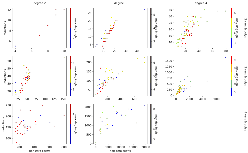
Simply counting the number of non-zero entries in a voo throws away quite a bunch of information. A different idea is to count the number of all non-zero coefficients in all the polynomials in $\mathcal{V}$. Continuing above example, that’d give a value of $15$. This approach might capture the complexity of computing a Gröbner basis more accurately, in part because large and involved $\mathcal{V}$s don’t just get squeezed into the interval $[0,1]$. The figure below suggests a correlation between the complexity of computing a Gröbner basis and the total number of non-zero coefficients in all voos, but it is still quite noisy.
The total number of non-zero coefficients in all vectors of origin vs the number of required reductions before a Gröbner basis is computed for random, determined systems of various sizes and of various degrees.
Including the Degree of the Voos
It is tempting to somehow mix the degrees of the voos into the involvement metric. However, I have not yet found a good way to do so, partly because the degrees of the voos can be very large even for very easy Gröbner basis computations.
For example, take $\mathcal{F}_{10} = ( x^{10}y + 1, xy^{10} )$. The reduced Gröbner basis for $\mathcal{F}$ is $\{1\}$, i.e., $\langle \mathcal{F} \rangle = \mathbb{F}[x, y]$. However, the two polynomials in the single vector of origin are both of degree $99$, far bigger than the Macaulay bound, which is $21$. In total, $10$ reductions are required to find the reduced Gröbner basis.
For system $\mathcal{F}_{100} = ( x^{100}y + 1, xy^{100} )$, the reduced Gröbner basis is still $\{1\}$. The Macaulay bound has increased to $201$, but the degrees of the two polynomials in the vector of origin is now $9999$, even though only $100$ reductions were required to compute the reducer Gröbner basis!
The degrees of the polynomials in the voos might not be of any practical relevance – at least, I haven’t spotted one yet. The argument might even be irrelevant for polynomial systems derived from a cryptographic primitive, since above examples might only work because $1$ is in the ideal spanned by $\mathcal{F}_{10}$ and $\mathcal{F}_{100}$.
Conclusion
Above ideas are still rather rough and need to be developed quite a bit before they can be useful. Regardless, I believe they might be a step in the direction for developing a lower bound for the complexity of computing a Gröbner basis of a given polynomial system. Or if not that, then maybe a heuristic, another tool for primitive designers to argue resistance against Gröbner basis attacks.
Cryptographic primitives designed to be algebraically simple – AOCs – might be particularly vulnerable to algebraic attacks. One of the most threatening attack vectors in this category is the Gröbner basis analysis. For a cipher or hash function to be considered secure, the Gröbner basis for any polynomial system derivable from the primitive needs to be intractable to compute.
Unfortunately, the complexity of computing a Gröbner basis for a specific polynomial system is generally not known before the computation is completed. However, some complexity bounds exist. One of the most prominently used bounds is based on a polynomial system’s degree of regularity.
Generally, computing the degree of regularity for a polynomial system is as hard as computing the Gröbner basis itself. Luckily, for an “average” regular determined system, the degree of regularity equals the Macaulay bound. That is, for $\mathcal{F} = \{f_0, \dots, f_{s-1}\} \subseteq \mathbb{F}[x_0, \dots, x_{n-1}]$ we have $d_\text{reg} = 1 + \sum_{i=0}^{s-1}\deg(f_i) – 1$.
How Current AOCs Argue Resistance to Gröbner Basis Analysis
The Poseidon [6] paper mentions the Macaulay bound, and implicitly assumes that the polynomial system arising from Poseidon is a regular sequence. My own experiments indicate that this assumption is false. Similarly, GMiMC [1] uses the Macaulay bound and assumes the regularity of the system implicitly. My own experiments indicate that this assumption is also false. The authors of Ciminion [4] explicitly assume the derived system to be regular, but mistakenly describe this to be “the best adversarial scenario” where in fact the opposite is true. Furthermore, my own experiments indicate that the polynomial sequence is not regular. For Rescue [2], the authors perform Gröbner basis attacks on round-reduced variants, showing that the system arising from Rescue is not regular. They then extrapolate the observed degrees to estimate the degree of regularity for the full-round primitive.
In summary, two approaches can be observed: (1) assume regularity of the system, then use the Macaulay bound to compute the degree of regularity, or (2) extrapolate the degree of regularity from round-reduced variants. Both approaches then use the degree of regularity to estimate the complexity for computing the Gröbner basis. This is generally done by looking at the complexity bound of the most efficient Gröbner basis algorithm, F5. This bound is $$O\left(\binom{n + d_\text{reg}}{n}^\omega\right)$$ where $n$ is the number of variables in the polynomial ring [3].
But: this is an upper bound. We need a lower bound.
The Degree of Regularity does not Suffice
I’ll make a series of increasingly complex and decreasingly pathological examples why the degree of regularity derived from the Macaulay bound does not suffice to accurately estimate the concrete complexity of computing a Gröbner basis. The ideals of all the systems below are of dimension $0$, meaning that the respective sets of common solutions are non-empty and contain finitely many elements. This accurately reflects the properties of polynomial systems modeling a cryptographic primitive.
The system is already a Gröbner basis
Let’s say we want to compute the Gröbner basis for $\mathcal{F}_\text{gb} = \{x^7, y^7, z^7\} \subseteq \mathbb{F}[x,y,z]$. We quickly see that $\mathcal{F}$ is a regular sequence, and determine that the degree of regularity is $d_\text{reg} = 1 + \sum_{i=0}^2 7 – 1 = 19$. Consequently, or so the roughly sketched argument above goes, a Gröbner basis algorithm like F4 or F5 should have to perform computations on polynomials of up to degree $19$ before being able to output a Gröbner basis.
However, $\mathcal{F}_\text{gb}$ is already a Gröbner basis – no computation at all is required!
The system can be split up
Deriving a polynomial system from a cryptographic primitive rarely gives you a Gröbner basis – although there are exceptions, like GMiMC. Instead, let’s look at the following polynomial system. $$\mathcal{F}_\text{indep} = \left\{\begin{aligned} &u^2 v w + u^2, && x^2 y z + x^2,\\ &u v^2 w + v^2 + 1, && x y^2 z + y^2 + 1,\\ &u v w^2 + w^2, && x y z^2 + z^2\\ \end{aligned}\right\} \subseteq \mathbb{F}[u,v,w,x,y,z].$$
The polynomials containing variables $u$, $v$ and $w$ are completely independent from the polynomials where $x$, $y$, and $z$ make an appearance. For the Macaulay bound, this fact is irrelevant. Since $\mathcal{F}_\text{indep}$ is a regular sequence, we might derive $d_\text{reg} = 1 + \sum_{i=0}^5 4 – 1 = 19$.
However, the F4 implementations of magma and FGb as well as the python implementation of F5 all compute on polynomials of only degree $5$ and lower before finding the Gröbner basis – they are not fooled by this attempt to artificially increase the complexity.
The system is not very “involved”
When deriving a polynomial system from a (single) cryptographic primitive, a partition in the set of polynomials like above is unlikely to appear – intuitively, that would lead to weak diffusion. Let’s change the system a little, then.$$ \mathcal{F}_\text{invlv} = \left\{ \begin{aligned} &u^2 v w + u^2, && x^2 y z + x^2,\\ &u v^2 w + v^2 + 1, && x y^2 z + y^2 + 1,\\ &u v w^2 + w^2, && u^4 + z^4\\ \end{aligned} \right\} \subseteq \mathbb{F}[u,v,w,x,y,z].$$
The sets $\mathcal{F}_\text{indep}$ and $\mathcal{F}_\text{invlv}$ differ in one polynomial, and this polynomial $(u^4 + z^4) = f_\text{link}$ links the two independent subsets of $\mathcal{F}_\text{indep}$. I didn’t derive the system from any concrete primitive, but a polynomial like $f_\text{link}$ might express how to move from one round to the next in a cipher.
The Macaulay bound for $\mathcal{F}_\text{invlv}$ does not change from the bound for $\mathcal{F}_\text{indep}$ since $f_\text{link}$ is of the same degree as the polynomial it replaced. Also, $\mathcal{F}_\text{invlv}$ is still a regular sequence, so we still have $d_\text{reg} = 19$.
You might have guessed it by now: the highest polynomials appearing during a Gröbner basis computation for $\mathcal{F}_\text{invlv}$ is not $19$. Magma’s F4 reports a maximum degree of $6$, FGb only reaches degree $5$, and so does python-F5.
While I don’t fully understand why this happens, vectors of origin give some hints. Briefly, $v_i$ is a vector of origin for Gröbner basis element $g_i$ if $\mathcal{F}_\text{invlv} \cdot v_i = g_i$. Below are the vectors of origin for $\mathcal{F}_\text{invlv}$, where any big polynomial is replaced by $\bullet$ to ease reading. $$\begin{align} &(\bullet, \bullet, {\small 0}, {\small 0}, {\small 0}, {\small 0}),\\ &(\bullet, \bullet, {\small 0}, {\small 0}, {\small 0}, {\small 0}),\\ &({\small 0}, {\small 0}, \bullet, 3, {\small 0}, {\small 0}),\\ &({\small 0}, {\small 0}, \bullet, \bullet, {\small 0}, {\small 0}),\\ &({\small 0}, {\small 0}, \bullet, \bullet, 1, {\small 0}),\\ &({\small 0}, {\small 0}, \bullet, \bullet, \bullet, 1)\\ \end{align}$$
A zero in position $i$ in a vector of origin means that $f_i$ was unnecessary for computing the Gröbner basis element. Above vectors of origin have a lot of zeros – in fact, even though all polynomials are linked to one another in some (potentially indirect) way, there seems to be a partition.
I describe polynomial systems for which the Gröbner bases’ elements can be computed from a few input polynomials at a time as having low “involvement.” As of yet, there is no mathematically rigourous way to define this notion, but above example should give a rough intuition. My observations indicate that low involvement means low complexity for computing a Gröbner basis.
Note. Above counter-examples do not disprove the equality of the degree of regularity and the Macaulay bound for generic polynomial systems – they only show that regularity of the sequence is not a sufficient requirement.
Existing Lower Bounds
The main message of this post is that we need (tight-ish) lower, not upper, bounds for estimating the complexity of a Gröbner basis computation in order to accurately asses the security of cryptographic primitives against this vector of attack. Unfortunately, the scientific literature currently has little to offer in this regard.
Hyun [5] exclusively deals with field $\mathbb{Q}$, while we are interested in finite fields, and Möller & Mora [7] look at ideals of positive dimension, while we are only interested in zero-dimensional ideals. Furthermore, all given bounds are existential while we need a constructive bound.
In summary, current strategies for arguing that some Arithmetization Oriented Primitive is resistant against Gröbner basis attacks make too many unbacked assumptions, often implicitly. The tools to make these arguments rigorously don’t currently exist. Or in other words: “look at me still talking when there’s science to do.”
References
Albrecht, M.R., Grassi, L., Perrin, L., Ramacher, S., Rechberger, C., Rotaru, D.,Roy, A., Schofnegger, M.: Feistel Structures for MPC, and More. In: ESORICS. pp.151–171. Springer (2019)
Aly, A., Ashur, T., Ben-Sasson, E., Dhooghe, S., Szepieniec, A.: Design of Symmetric Primitives for Advanced Cryptographic Protocols. IACR ToSC 2020(3), 1–45(2020)
Bardet, M., Faugère, J.C., Salvy, B.: On the complexity of the F5 Gröbner basis algorithm. Journal of Symbolic Computation 70, 49–70 (2015)
Dobraunig, C.E., Grassi, L., Guinet, A., Kuijsters, D.: Ciminion: Symmetric Encryption Based on Toffoli-Gates over Large Finite Fields. In: Eurocrypt 2021 (2021)
Huynh, Dung T.: A superexponential lower bound for Gröbner bases and Church-Rosser commutative Thue systems. Information and Control, 68(1- 3):196–206 (1986)
Grassi, L., Khovratovich, D., Rechberger, C., Roy, A., Schofnegger, M.: Poseidon: A New Hash Function for Zero-Knowledge Proof Systems. In: USENIX Security. USENIXAssociation (2020)
Möller, H. M., and Mora, F.: Upper and lower bounds for the degree of Gröbner bases. In: International Symposium on Symbolic and Algebraic Manipulation, pages 172–183. Springer (1984)
Computing the degree of regularity for a regular sequence spanning a zero-dimensional ideal is easy – the Macaulay bound is the answer we’re looking for. If the polynomial system does not meet these conditions, the problem is a little more intricate. Concretly: computing the degree of regularity for a polynomial system is generally as difficult as computing its Gröbner basis.
This might suggest that computing the degree of regularity from a Gröbner basis is easy. After all, we’ve done all the hard work already! Unfortunately, this is not generally the case, as the following example will make clear.
In this blog post, I will use “degree of regularity” and ”highest degree reached during computation of the Gröbner basis” interchangeably. While this is not true in general, the degrees are close enough for the argument below to be valid still.
Consider the system $\mathcal{F} = \{ x^2 y + 1, x y^2 \} \subseteq \mathbb{F}[x, y]$ for some finite field $\mathbb{F}$. Let’s start computing the Gröbner basis for degrevlex order using Buchberger’s algorithm:
Keeping track, we computed a polynomial of degree 4, even though the highest degree monomial didn’t make it into the end result. One more step and we’ve found the Gröbner basis:
Seems like $\mathcal{F}$ is inconsistent – the reduced Gröbner basis of $\mathcal{F}$ is $\{1\}$, meaning the variety of $\langle \mathcal{F} \rangle$ is empty. Good to know. The degree of regularity of $\mathcal{F}$ is 4, reached during computation of the first S-Polynomial.
Already it becomes apparent that computing the degree of regularity from this Gröbner basis is impossible. Let me drive home the point by considering $\mathcal{F}_a = \{x^a y + 1, xy^a\}$ for positive integer $a$. It is easy to see that the reduced Gröbner basis of $\mathcal{F}_a$ is $\{1\}$ for any $a$. However, the degree of the highest degree polynomial appearing during computation of said Gröbner basis – whether using Buchberger’s algorithm, F4, F5, or Mutant XL – is $2a$.
Identifying classes of polynomial systems for which the degree of regularity can easily be deduced from its Gröbner basis is an interesting question. Are consistent systems such a class? Consistent systems spanning a zero-dimensional ideal? Does regularity of the system play a role? The example above has only shown that it is impossible in general.
Any cryptographic primitive – cipher, hash function, etc. – can be expressed through multivariate polynomial equations. An efficient way to solve these equations simultaneously breaks the underlying primitive. Gröbner bases are a great way to simultaneously solve multiple multivariate polynomial equations. For more details on this, have a look at our previous post on Gröbner basis attacks.
Someone designing a cryptographic primitive has to show or convincingly argue resilience against any applicable vector of attack, one of which are Gröbner basis attacks. Whether or not actually computing a Gröbner basis for a specific system is realistically achievable before the heat death of the universe depends on a number of factors. The designer of the primitive needs to show or argue that all systems derived from their primitive are not “easy.”
What is this Degree of Regularity?
Computing a Gröbner basis from a system of polynomials is hard on average – but how hard exactly is difficult to know before completing the computation. The degree of regularity of a system of polynomials is a value with which an upper bound on the complexity can be derived. Concretely, computing a Gröbner basis for a system of polynomials $\mathcal{F}$ over multivariate ring $R[x_0, \dots, x_{n-1}]$ has complexity in $$O {\Big(} \binom{n + d_{\text{reg}}}{n} ^ \omega {\Big)}.$$ The linear algebra constant $\omega$ is a value between 2 and 3 and depends on the implementation of matrix multiplication. The degree of regularity $d_{\text{reg}}$ depends on $\mathcal{F}$ in intricate ways.
An intuitive understanding
I will intuit one possible derivation of the degree of regularity using an example. You can find some self-contained sagemath code at the bottom of this post, implementing the example. The code is generic enough that you can use any ring and polynomial system you want, and I encourage you to play around with it. Note that the code is written for readability, not for performance; if you want to compute a Gröbner basis in earnest, try sagemath’s groebner_basis() function, or use even more specialized tools.
A polynomial system
Let \begin{align} \mathcal{F} = \{& xz + 3y, \\ & y + z + 2, \\ & xy + y^2 \} \end{align} over tri-variate ring $\mathbb{F}_{101}[x, y, z]$. To find the degree of regularity of $\mathcal{F}$, we will compute its Gröbner basis. One rather inefficient but insightful way to compute a Gröbner basis is to triangulize the Macaulay matrix of $F$ for a high enough degree. In fact, the smallest degree that is high enough is precisely the degree of regularity. But first, let’s transform polynomials into vectors.
Polynomials as vectors
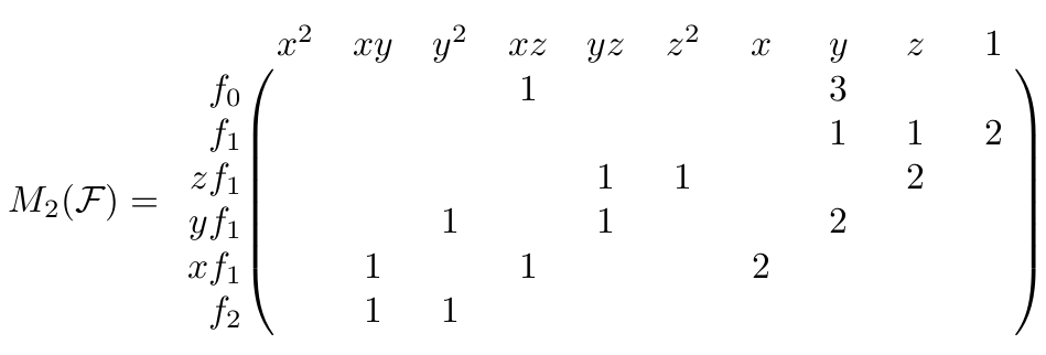
It is possible to identify a polynomial of a fix degree with a vector with entries only in the base field. Take $f = xz + 3y$, for example. The total degree of $f$ is 2. All possible monomials in 3 variables of degree 2 or less are $$\boldsymbol{m} = (x^2, xy, y^2, xz, yz, z^2, x, y, z, 1).$$ Using vector $\boldsymbol{a} = (0, 0, 0, 1, 0, 0, 0, 3, 0, 0)$, we have $\boldsymbol{m}\cdot\boldsymbol{a}^\intercal = f$. Note that the elements of $\boldsymbol{a}$ come from the base field $\mathbb{F}_{101}$. This allows us to perform linear algebra operations, for which fast techniques and tools exist.
The Macaulay matrix
The Macaulay matrix of degree $d$ contains all monomial multiples of the elements of $\mathcal{F}$ such that the degree of any such product is not greater than $d$. More formally, we perform the following steps.
M = ∅
for each polynomial f in F:
    for each monomial m with deg(m) ≤ d - deg(f):
        v = poly_to_vec(m·f)        // pad with zeros as needed
        M = M ∪ {v}
mac_mat = matrix(M)
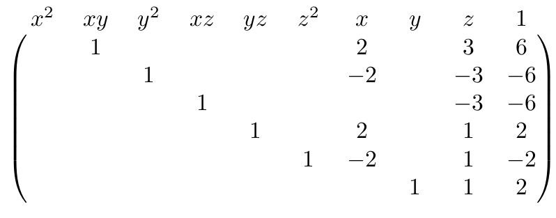
Building the Macaulay matrix of degree 2 for above system $\mathcal{F}$, we get the following matrix $M_2(\mathcal{F})$. For convenience, I have labeled the rows with the polynomials and the columns with the monomials they each correspond to. To reduce visual clutter, zeros are not printed.
Sidenote: I’m brushing over monomial orders right now, which is a concept central to Gröbner basis computations. In this post, we’re only using degrevlex, but the steps work with any graded order.
Triangularizing the Macaulay matrix
Since scalar multiplications and additions of polynomials within a polynomial system do not change the ideal they span, we can simplify $M_2(\mathcal{F})$ by building its row-reduced echelon form. Note that exchanging columns is not permitted, since that would alter the order of the monomials, and that means bad things can happen. (The generalization of Gröbner basis computations where, in some cases, swapping columns is allowed, are called dynamic Gröbner basis algorithms.)
Triangularizing $M_2(\mathcal{F})$ using only row-operations leads to the following matrix:
Interpreting the rows as polynomials again, we get the following set $G_2$.\begin{align*}G_2 = \{&xy + 2x + 3z + 6, \\&y^2 – 2x – 3z – 6, \\&xz – 3z – 6, \\&yz + 2x + z + 2, \\&z^2 – 2x + z – 2, \\&y + z + 2\}\end{align*}
Removing redundancies
Some of the elements in $G_2$ are redundant for the ideal $\langle G_2 \rangle$. For example, $\langle G_2 \rangle$ and the ideal spanned by $G_2 \setminus \{xy + 2x + 3z + 6\}$ are the same: We can “build” $(xy + 2x + 3z + 6) = x(y + z + 2) – (xz – 3z – 6)$ from other polynomials in $G_2$.
Removing all redundant elements like this, we end up with $G’_2$.\begin{align*}G’_2 = \{&xz – 3z – 6, \\&z^2 – 2x + z – 2, \\&y + z + 2\}\end{align*}
Checking the result
The burning question: Is $G’_2$ a Gröbner basis for $\langle \mathcal{F} \rangle$? Let’s start applying the Buchberger criterion by building S-Polynomials.
Polynomial division of $g_0$ by $G’_2$ leaves remainder $2x^2 – 4x – 6z – 12$. This is not 0, meaning that $G’_2$ is not a Gröbner basis! Bummer. Let’s try the same steps with a bigger Macaulay matrix, going to degree 3.
Raising the degree for the Macaulay matrix
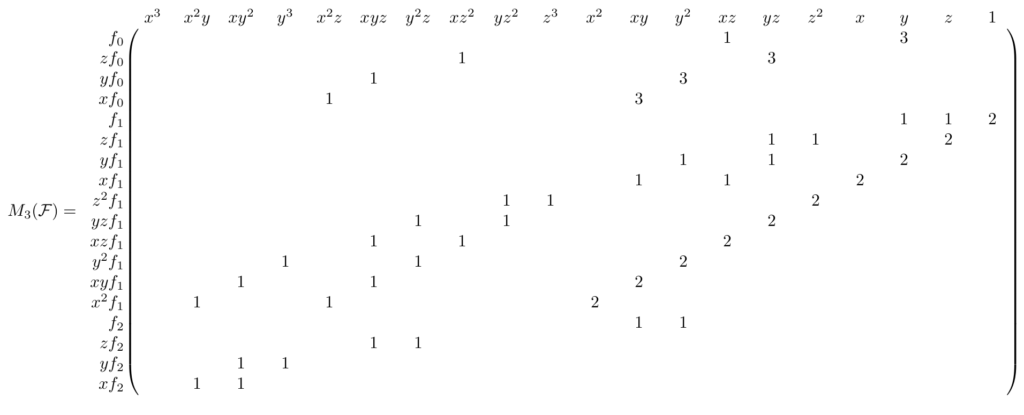
The Macaulay matrix of degree 3 for our system of polynomials $\mathcal{F}$ looks as follows.
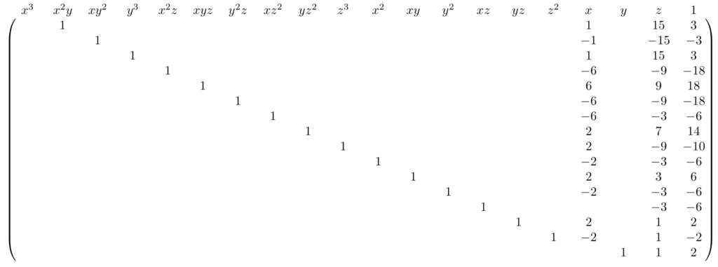
Wow, this has grown! And no wonder: the number of monomials below degree $d$ for a fix number of variables – 3 in our case – grows factorially with $d$. Anyway, the triangulated matrix (with all zero-rows removed) looks a little like this:
The rows of this matrix correspond to the polynomials in set $G_3$.
Again, we remove redundant polynomials, resulting in $G’_3$. This is only one element bigger than $G’_2$! But this one missing element did the trick: $G’_3$ is a Gröbner basis, spanning the same ideal as $\mathcal{F}$.
Note: $G_3$ is also a Gröbner basis for $\langle \mathcal{F} \rangle$, but $G’_3$ is the (unique) reduced Gröbner basis.
The Degree of Regularity
The highest degree of any of the elements in $\mathcal{F}$ is $2$. The same is true for its Gröbner basis $G’_3$. However, in order to compute $G’_3$ from $\mathcal{F}$, we needed to work with polynomials of degree $3$ – the Macaulay matrix $M_2(\mathcal{F})$ of degree 2 did not suffice.
Even though this is not the formal definition, the degree of regularity is the lowest degree for which triangularizing the Macaulay matrix results in a Gröbner basis.
Except in the special case of regular systems, computing the degree of regularity is as hard as computing the Gröbner basis itself – even using more advanced algorithms like F₄ or F₅. This is quite annoying when you want to use the degree of regularity to determine how hard a Gröbner basis computation might get! Luckily, many polynomial systems encountered “in the wild” are in fact regular.
Please note that the degree of regularity allows deriving an upper bound for the complexity of computing a Gröbner basis. Arguing that the compution is difficult for some system by only talking about the degree of regularity is a great faux-pas! If the system behaves like a random one, the upper bound is tight and the argument stands.
Playtime! – Sagemath Code
def all_monoms_upto_deg(ring, d):
    all_monoms = set()
    last_monoms = [ring(1)]
    for i in range(d):
        all_monoms.update(last_monoms)
        last_monoms = [l*v for l in last_monoms for v in ring.gens()]
    all_monoms.update(last_monoms)
    return sorted(all_monoms)[::-1]

def macaulay_matrix(polys, d):
    ring = polys[0].parent()
    columns = all_monoms_upto_deg(ring, d)
    mm_pols = []
    for p in polys:
        factors = [f for f in columns if f.lm()*p.lm() in columns]
        factors = factors[::-1] # original polynomial in highest possible row
        mm_pols += [f*p for f in factors]
    mm_rows = [[p.monomial_coefficient(c) for c in columns] for p in mm_pols]
    return matrix(mm_rows)

def gauss_elimination(A):
    A = copy(A)
    nrows, ncols = A.nrows(), A.ncols()
    for c in range(ncols):
        for r in range(nrows):
            if A[r,c] and not any(A[r,i] for i in range(c)):
                a_inverse = ~A[r,c]
                A.rescale_row(r, a_inverse)
                for i in range(nrows):
                    if i != r and A[i,c]:
                        minus_b = -A[i,c]
                        A.add_multiple_of_row(i, r, minus_b)
                break
    empty_rows = [i for i in range(nrows) if not any(A.row(i))]
    A = A.delete_rows(empty_rows)
    A = matrix(sorted(A)[::-1])
    return A

def polynomial_division(f, divisors):
    f_original = f
    quotients = [0]*len(divisors)
    rem = 0
    while f != 0:
        i = 0
        division_occured = False
        while i < len(divisors) and not division_occured:
            divisable = False
            try:
                divisable = divisors[i].lt().divides(f.lt())
            except NotImplementedError as e:
                pass # _beautiful_ solution
            if divisable:
                q, _ = f.lt().quo_rem(divisors[i].lt())
                quotients[i] += q
                f = f - q * divisors[i]
                division_occured = True
            else:
                i += 1
        if not division_occured:
            r = f.lt()
            rem += r
            f -= r
    assert f_original == sum([q*d for q, d in zip(quotients, divisors)]) + rem
    return quotients, rem

def interreduce(polys):
    i = 0
    while i < len(polys):
        reductee = polys[i]
        polys_wo_reductee = [p for p in polys if p != reductee]
        _, rem = polynomial_division(reductee, polys_wo_reductee)
        if not rem:
            polys = polys_wo_reductee
            i = 0
        else:
            i += 1
    return polys

def s_poly(f, g):
    l = f.lm().lcm(g.lm())
    factor_f = l // f.lt()
    factor_g = l // g.lt()
    return factor_f * f - factor_g * g

def buchberger_criterion(gb):
    for j in range(len(gb)):
        for i in range(j):
            s = s_poly(gb[i], gb[j])
            _, rem = polynomial_division(s, gb)
            if rem:
                return False
    return True

if __name__ == "__main__":
    ring.<x,y,z> = GF(101)[]
    polys = [x*z + 3*y, y + z + 2, x*y + y^2]
    print(f"Ring: {ring}")
    print(f"Input polynomials:\n{polys}")
    d = 0
    is_gb = False
    while not is_gb:
        columns = vector(all_monoms_upto_deg(ring, d))
        mm = macaulay_matrix(polys, d)
        ge = gauss_elimination(mm)
        gb = [row * columns for row in ge]
        gb_red = interreduce(gb)
        quos_rems = [polynomial_division(p, gb_red) for p in polys]
        rems = [r for _, r in quos_rems]
        is_gb = buchberger_criterion(gb_red) and not any(rems)

        print(f"\n––– Degree {d} –––")
        print(f"Macaulay matrix:\n{mm}")
        print(f"Echelon row-reduced Macaulay matrix:\n{ge}")
        print(f"Polynomials in echelon row-reduced Macaulay matrix:\n{gb}")
        print(f"Without redundancies:\n{gb_red}")
        print(f"Is Gröbner Basis: {is_gb}")
        if not is_gb: d += 1
    gb_sage = Ideal(polys).groebner_basis()
    assert sorted(gb_red) == sorted(gb_sage),\
        f"We did not compute the reduced Gröbner basis"
    print(f"Degree of regularity: {d}")