Why We Need New Metrics

In my last post, I’ve argued against the use of degree of regularity-based bounds for conservatively estimating the complexity of a Gröbner basis attack. In a nutshell, all these bounds are upper bounds, where we really need lower bounds.

For example, consider the polynomial system $\mathcal{F} = \{f_0, f_1, f_2\} \subseteq \mathbb{F}[x, y, z]$ for some finite field $\mathbb{F}$ with\[f_0 = x^{100}z + y, \qquad f_1 = x, \qquad f_2 = z \;.\] Independent of the monomial order, the reduced Gröbner basis of $\mathcal{F}$ is $\mathcal{G} = \{x, y, z\}$. The degree of regularity of $\mathcal{F}$ is $101 = \deg(f_0)$. The Macaulay bound for $\mathcal{F}$ is equal to the degree of regularity. Looking only at these numbers might give the impression that computing $\mathcal{G}$ is difficult. However, after constructing just one S-Polynomial $f_0 – x^{100} \cdot f_2 = y$, the Gröbner basis is already computed. All that’s left is reducing now redundant $f_0$, and we have the reduced Gröbner basis, $\mathcal{G}$.

Vectors of Origin – Explaining GBs

The connections between polynomials of some system $\mathcal{F}$ and its Gröbner basis $\mathcal{G}$ are usually not clear at all. For example, consider $$\mathcal{F} = (x^2 + z^2, z^2t + t, xy^2 + y + 1, x^2y + x)$$ and its reduced Gröbner basis $$\mathcal{G} = (x, y + 1, z^2, t).$$ Which input element was required for which Gröbner basis elements? Can some Gröbner basis elements be derived by using only a subset of the input? How were the input elements combined?

Vectors of origin (voo) answer these – and potentially more – questions. A voo $\mathbf{v} \in \mathbb{F}[x_0, \dots, x_{n-1}]^{|\mathcal{F}|}$ for some Gröbner basis element $g \in \mathcal{G}$ is a vector of polynomials such that $\mathcal{F} \cdot \mathbf{v} = g$. For example, $(0, 0, x, -y)$ is the voo for $x \in \mathcal{G}$. Arranging all voo’s into matrix $\mathcal{V}$, we have $\mathcal{F} \cdot \mathcal{V} = \mathcal{G}$. This $n\times |\mathcal{F}|$ matrix, where each entry is a multivariate polynomial, contains a lot of juicy information about $\mathcal{F}$.

We can compute voos by tweaking Gröbner basis algorithm F₅. F₅ uses signatures to avoid many useless reductions – and a signature is essentially derived from a voo, even though the voo is usually not computed explicitly. By modifying existing code for F₅ slightly, we can thus easily get $\mathcal{V}$ in addition to $\mathcal{G}$.

Involvement of the Input System

An element $g$ of a Gröbner basis is not necessarily the polynomially weighted sum of all input polynomials, as the examples above show. I have dreamed up a metric measuring how many elements of a reduced Gröbner basis rely on how many input system elements. Its working title is the ”involvement” metric. It’s not finished, but you might find the ideas interesting.

The involvement of some system $\mathcal{F}$ is the normalized measure of how many elements of $\mathcal{G}$ depend on how many polynomials in $\mathcal{F}$. More precisely, denote the number of non-zero entries in voo $\mathbf{v}_i$ by $v_i$. The mean of all $v_i$’s is the mean number of input elements making up the Gröbner basis elements. Since every Gröbner basis element is the combination of at least one input polynomial, we can safely subtract $1$ from $v_i$ before taking the mean, without losing information. This has the added benefit that the involvement metric is $0$ if the input is a Gröbner basis, since the vectors of origin will be (a subset of) the identity vectors. Normalizing this mean, i.e., dividing it by $|\mathcal{F}| – 1$ such that the result is in the interval $[0, 1]$, then gives the involvement metric. This sagemath one-liner below captures this description more concisely:

mean([sum([1 for v in voo if v])-1 for voo in V]) / (len(F)-1)

Let’s return to the example above. The matrix $\mathcal{V}$ with all vectors of origin is $$\mathcal{V} = \left(\begin{matrix} 0 & 0 & x & -y \\ 1 & 0 & -x^2 & xy \\ 0 & 0 & -xy^2+1 & y^3 \\ -xyt-t & xy+1 & -xyt & y^2t+xt \\ \end{matrix}\right).$$ We have $v_0 = v_2 = 2$, $v_1 = 3$, and $v_3 = 4$. The mean is $\frac{\sum v_i – 1}{4} = \frac{7}{4}$, normalizing (in this case) corresponds to a division by $3$, so the result is $\frac{7}{12} \approx 0.583$.

Involvement as Number of Non-Zero Coefficients

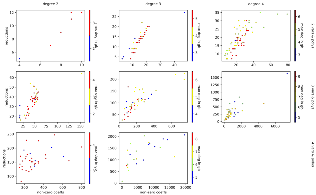
Simply counting the number of non-zero entries in a voo throws away quite a bunch of information. A different idea is to count the number of all non-zero coefficients in all the polynomials in $\mathcal{V}$. Continuing above example, that’d give a value of $15$. This approach might capture the complexity of computing a Gröbner basis more accurately, in part because large and involved $\mathcal{V}$s don’t just get squeezed into the interval $[0,1]$. The figure below suggests a correlation between the complexity of computing a Gröbner basis and the total number of non-zero coefficients in all voos, but it is still quite noisy.

Including the Degree of the Voos

It is tempting to somehow mix the degrees of the voos into the involvement metric. However, I have not yet found a good way to do so, partly because the degrees of the voos can be very large even for very easy Gröbner basis computations.

For example, take $\mathcal{F}_{10} = ( x^{10}y + 1, xy^{10} )$. The reduced Gröbner basis for $\mathcal{F}$ is $\{1\}$, i.e., $\langle \mathcal{F} \rangle = \mathbb{F}[x, y]$. However, the two polynomials in the single vector of origin are both of degree $99$, far bigger than the Macaulay bound, which is $21$. In total, $10$ reductions are required to find the reduced Gröbner basis.

For system $\mathcal{F}_{100} = ( x^{100}y + 1, xy^{100} )$, the reduced Gröbner basis is still $\{1\}$. The Macaulay bound has increased to $201$, but the degrees of the two polynomials in the vector of origin is now $9999$, even though only $100$ reductions were required to compute the reducer Gröbner basis!

The degrees of the polynomials in the voos might not be of any practical relevance – at least, I haven’t spotted one yet. The argument might even be irrelevant for polynomial systems derived from a cryptographic primitive, since above examples might only work because $1$ is in the ideal spanned by $\mathcal{F}_{10}$ and $\mathcal{F}_{100}$.

Conclusion

Above ideas are still rather rough and need to be developed quite a bit before they can be useful. Regardless, I believe they might be a step in the direction for developing a lower bound for the complexity of computing a Gröbner basis of a given polynomial system. Or if not that, then maybe a heuristic, another tool for primitive designers to argue resistance against Gröbner basis attacks.

Cryptographic primitives designed to be algebraically simple – AOCs – might be particularly vulnerable to algebraic attacks. One of the most threatening attack vectors in this category is the Gröbner basis analysis. For a cipher or hash function to be considered secure, the Gröbner basis for any polynomial system derivable from the primitive needs to be intractable to compute.

Unfortunately, the complexity of computing a Gröbner basis for a specific polynomial system is generally not known before the computation is completed. However, some complexity bounds exist. One of the most prominently used bounds is based on a polynomial system’s degree of regularity.

Generally, computing the degree of regularity for a polynomial system is as hard as computing the Gröbner basis itself. Luckily, for an “average” regular determined system, the degree of regularity equals the Macaulay bound. That is, for $\mathcal{F} = \{f_0, \dots, f_{s-1}\} \subseteq \mathbb{F}[x_0, \dots, x_{n-1}]$ we have $d_\text{reg} = 1 + \sum_{i=0}^{s-1}\deg(f_i) – 1$.

How Current AOCs Argue Resistance to Gröbner Basis Analysis

The Poseidon [6] paper mentions the Macaulay bound, and implicitly assumes that the polynomial system arising from Poseidon is a regular sequence. My own experiments indicate that this assumption is false. Similarly, GMiMC [1] uses the Macaulay bound and assumes the regularity of the system implicitly. My own experiments indicate that this assumption is also false. The authors of Ciminion [4] explicitly assume the derived system to be regular, but mistakenly describe this to be “the best adversarial scenario” where in fact the opposite is true. Furthermore, my own experiments indicate that the polynomial sequence is not regular. For Rescue [2], the authors perform Gröbner basis attacks on round-reduced variants, showing that the system arising from Rescue is not regular. They then extrapolate the observed degrees to estimate the degree of regularity for the full-round primitive.

In summary, two approaches can be observed: (1) assume regularity of the system, then use the Macaulay bound to compute the degree of regularity, or (2) extrapolate the degree of regularity from round-reduced variants. Both approaches then use the degree of regularity to estimate the complexity for computing the Gröbner basis. This is generally done by looking at the complexity bound of the most efficient Gröbner basis algorithm, F₅. This bound is $$O\left(\binom{n + d_\text{reg}}{n}^\omega\right)$$ where $n$ is the number of variables in the polynomial ring [3].

But: this is an upper bound. We need a lower bound.

The Degree of Regularity does not Suffice

I’ll make a series of increasingly complex and decreasingly pathological examples why the degree of regularity derived from the Macaulay bound does not suffice to accurately estimate the concrete complexity of computing a Gröbner basis. The ideals of all the systems below are of dimension $0$, meaning that the respective sets of common solutions are non-empty and contain finitely many elements. This accurately reflects the properties of polynomial systems modeling a cryptographic primitive.

The system is already a Gröbner basis

Let’s say we want to compute the Gröbner basis for $\mathcal{F}_\text{gb} = \{x^7, y^7, z^7\} \subseteq \mathbb{F}[x,y,z]$. We quickly see that $\mathcal{F}$ is a regular sequence, and determine that the degree of regularity is $d_\text{reg} = 1 + \sum_{i=0}^2 7 – 1 = 19$. Consequently, or so the roughly sketched argument above goes, a Gröbner basis algorithm like F₄ or F₅ should have to perform computations on polynomials of up to degree $19$ before being able to output a Gröbner basis.

However, $\mathcal{F}_\text{gb}$ is already a Gröbner basis – no computation at all is required!

The system can be split up

Deriving a polynomial system from a cryptographic primitive rarely gives you a Gröbner basis – although there are exceptions, like GMiMC. Instead, let’s look at the following polynomial system. $$\mathcal{F}_\text{indep} = \left\{\begin{aligned} &u^2 v w + u^2, && x^2 y z + x^2,\\ &u v^2 w + v^2 + 1, && x y^2 z + y^2 + 1,\\ &u v w^2 + w^2, && x y z^2 + z^2\\ \end{aligned}\right\} \subseteq \mathbb{F}[u,v,w,x,y,z].$$

The polynomials containing variables $u$, $v$ and $w$ are completely independent from the polynomials where $x$, $y$, and $z$ make an appearance. For the Macaulay bound, this fact is irrelevant. Since $\mathcal{F}_\text{indep}$ is a regular sequence, we might derive $d_\text{reg} = 1 + \sum_{i=0}^5 4 – 1 = 19$.

However, the F₄ implementations of magma and FGb as well as the python implementation of F₅ all compute on polynomials of only degree $5$ and lower before finding the Gröbner basis – they are not fooled by this attempt to artificially increase the complexity.

The system is not very “involved”

When deriving a polynomial system from a (single) cryptographic primitive, a partition in the set of polynomials like above is unlikely to appear – intuitively, that would lead to weak diffusion. Let’s change the system a little, then.$$ \mathcal{F}_\text{invlv} = \left\{ \begin{aligned} &u^2 v w + u^2, && x^2 y z + x^2,\\ &u v^2 w + v^2 + 1, && x y^2 z + y^2 + 1,\\ &u v w^2 + w^2, && u^4 + z^4\\ \end{aligned} \right\} \subseteq \mathbb{F}[u,v,w,x,y,z].$$

The sets $\mathcal{F}_\text{indep}$ and $\mathcal{F}_\text{invlv}$ differ in one polynomial, and this polynomial $(u^4 + z^4) = f_\text{link}$ links the two independent subsets of $\mathcal{F}_\text{indep}$. I didn’t derive the system from any concrete primitive, but a polynomial like $f_\text{link}$ might express how to move from one round to the next in a cipher.

The Macaulay bound for $\mathcal{F}_\text{invlv}$ does not change from the bound for $\mathcal{F}_\text{indep}$ since $f_\text{link}$ is of the same degree as the polynomial it replaced. Also, $\mathcal{F}_\text{invlv}$ is still a regular sequence, so we still have $d_\text{reg} = 19$.

You might have guessed it by now: the highest polynomials appearing during a Gröbner basis computation for $\mathcal{F}_\text{invlv}$ is not $19$. Magma’s F₄ reports a maximum degree of $6$, FGb only reaches degree $5$, and so does python-F₅.

While I don’t fully understand why this happens, vectors of origin give some hints. Briefly, $v_i$ is a vector of origin for Gröbner basis element $g_i$ if $\mathcal{F}_\text{invlv} \cdot v_i = g_i$. Below are the vectors of origin for $\mathcal{F}_\text{invlv}$, where any big polynomial is replaced by $\bullet$ to ease reading. $$\begin{align} &(\bullet, \bullet, {\small 0}, {\small 0}, {\small 0}, {\small 0}),\\ &(\bullet, \bullet, {\small 0}, {\small 0}, {\small 0}, {\small 0}),\\ &({\small 0}, {\small 0}, \bullet, 3, {\small 0}, {\small 0}),\\ &({\small 0}, {\small 0}, \bullet, \bullet, {\small 0}, {\small 0}),\\ &({\small 0}, {\small 0}, \bullet, \bullet, 1, {\small 0}),\\ &({\small 0}, {\small 0}, \bullet, \bullet, \bullet, 1)\\ \end{align}$$

A zero in position $i$ in a vector of origin means that $f_i$ was unnecessary for computing the Gröbner basis element. Above vectors of origin have a lot of zeros – in fact, even though all polynomials are linked to one another in some (potentially indirect) way, there seems to be a partition.

I describe polynomial systems for which the Gröbner bases’ elements can be computed from a few input polynomials at a time as having low “involvement.” As of yet, there is no mathematically rigourous way to define this notion, but above example should give a rough intuition. My observations indicate that low involvement means low complexity for computing a Gröbner basis.

Note. Above counter-examples do not disprove the equality of the degree of regularity and the Macaulay bound for generic polynomial systems – they only show that regularity of the sequence is not a sufficient requirement.

Existing Lower Bounds

The main message of this post is that we need (tight-ish) lower, not upper, bounds for estimating the complexity of a Gröbner basis computation in order to accurately asses the security of cryptographic primitives against this vector of attack. Unfortunately, the scientific literature currently has little to offer in this regard.

Hyun [5] exclusively deals with field $\mathbb{Q}$, while we are interested in finite fields, and Möller & Mora [7] look at ideals of positive dimension, while we are only interested in zero-dimensional ideals. Furthermore, all given bounds are existential while we need a constructive bound.

In summary, current strategies for arguing that some Arithmetization Oriented Primitive is resistant against Gröbner basis attacks make too many unbacked assumptions, often implicitly. The tools to make these arguments rigorously don’t currently exist. Or in other words: “look at me still talking when there’s science to do.”

References

1. Albrecht, M.R., Grassi, L., Perrin, L., Ramacher, S., Rechberger, C., Rotaru, D.,Roy, A., Schofnegger, M.: Feistel Structures for MPC, and More. In: ESORICS. pp.151–171. Springer (2019)
2. Aly, A., Ashur, T., Ben-Sasson, E., Dhooghe, S., Szepieniec, A.: Design of Symmetric Primitives for Advanced Cryptographic Protocols. IACR ToSC 2020(3), 1–45(2020)
3. Bardet, M., Faugère, J.C., Salvy, B.: On the complexity of the F5 Gröbner basis algorithm. Journal of Symbolic Computation 70, 49–70 (2015)
4. Dobraunig, C.E., Grassi, L., Guinet, A., Kuijsters, D.: Ciminion: Symmetric Encryption Based on Toffoli-Gates over Large Finite Fields. In: Eurocrypt 2021 (2021)
5. Huynh, Dung T.: A superexponential lower bound for Gröbner bases and Church-Rosser commutative Thue systems. Information and Control, 68(1- 3):196–206 (1986)
6. Grassi, L., Khovratovich, D., Rechberger, C., Roy, A., Schofnegger, M.: Poseidon: A New Hash Function for Zero-Knowledge Proof Systems. In: USENIX Security. USENIXAssociation (2020)
7. Möller, H. M., and Mora, F.: Upper and lower bounds for the degree of Gröbner bases. In: International Symposium on Symbolic and Algebraic Manipulation, pages 172–183. Springer (1984)