The Degree of Regularity – Intuition using Linear Algebra
Why bother with Gröbner bases?
Any cryptographic primitive – cipher, hash function, etc. – can be expressed through multivariate polynomial equations. An efficient way to solve these equations simultaneously breaks the underlying primitive. Gröbner bases are a great way to simultaneously solve multiple multivariate polynomial equations. For more details on this, have a look at our previous post on Gröbner basis attacks.
Someone designing a cryptographic primitive has to show or convincingly argue resilience against any applicable vector of attack, one of which are Gröbner basis attacks. Whether or not actually computing a Gröbner basis for a specific system is realistically achievable before the heat death of the universe depends on a number of factors. The designer of the primitive needs to show or argue that all systems derived from their primitive are not “easy.”
What is this Degree of Regularity?
Computing a Gröbner basis from a system of polynomials is hard on average – but how hard exactly is difficult to know before completing the computation. The degree of regularity of a system of polynomials is a value with which an upper bound on the complexity can be derived. Concretely, computing a Gröbner basis for a system of polynomials $\mathcal{F}$ over multivariate ring $R[x_0, \dots, x_{n-1}]$ has complexity in $$O {\Big(} \binom{n + d_{\text{reg}}}{n} ^ \omega {\Big)}.$$ The linear algebra constant $\omega$ is a value between 2 and 3 and depends on the implementation of matrix multiplication. The degree of regularity $d_{\text{reg}}$ depends on $\mathcal{F}$ in intricate ways.
An intuitive understanding
I will intuit one possible derivation of the degree of regularity using an example. You can find some self-contained sagemath code at the bottom of this post, implementing the example. The code is generic enough that you can use any ring and polynomial system you want, and I encourage you to play around with it. Note that the code is written for readability, not for performance; if you want to compute a Gröbner basis in earnest, try sagemath’s groebner_basis() function, or use even more specialized tools.
A polynomial system
Let \begin{align} \mathcal{F} = \{& xz + 3y, \\ & y + z + 2, \\ & xy + y^2 \} \end{align} over tri-variate ring $\mathbb{F}_{101}[x, y, z]$. To find the degree of regularity of $\mathcal{F}$, we will compute its Gröbner basis. One rather inefficient but insightful way to compute a Gröbner basis is to triangulize the Macaulay matrix of $F$ for a high enough degree. In fact, the smallest degree that is high enough is precisely the degree of regularity. But first, let’s transform polynomials into vectors.
Polynomials as vectors
It is possible to identify a polynomial of a fix degree with a vector with entries only in the base field. Take $f = xz + 3y$, for example. The total degree of $f$ is 2. All possible monomials in 3 variables of degree 2 or less are $$\boldsymbol{m} = (x^2, xy, y^2, xz, yz, z^2, x, y, z, 1).$$ Using vector $\boldsymbol{a} = (0, 0, 0, 1, 0, 0, 0, 3, 0, 0)$, we have $\boldsymbol{m}\cdot\boldsymbol{a}^\intercal = f$. Note that the elements of $\boldsymbol{a}$ come from the base field $\mathbb{F}_{101}$. This allows us to perform linear algebra operations, for which fast techniques and tools exist.
The Macaulay matrix
The Macaulay matrix of degree $d$ contains all monomial multiples of the elements of $\mathcal{F}$ such that the degree of any such product is not greater than $d$. More formally, we perform the following steps.
M = ∅
for each polynomial f in F:
    for each monomial m with deg(m) ≤ d - deg(f):
        v = poly_to_vec(m·f)        // pad with zeros as needed
        M = M ∪ {v}
mac_mat = matrix(M)
Building the Macaulay matrix of degree 2 for above system $\mathcal{F}$, we get the following matrix $M_2(\mathcal{F})$. For convenience, I have labeled the rows with the polynomials and the columns with the monomials they each correspond to. To reduce visual clutter, zeros are not printed.
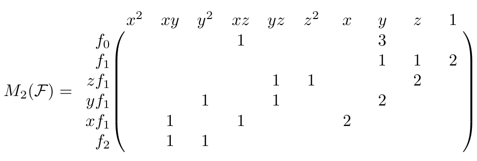
Sidenote: I’m brushing over monomial orders right now, which is a concept central to Gröbner basis computations. In this post, we’re only using degrevlex, but the steps work with any graded order.
Triangularizing the Macaulay matrix
Since scalar multiplications and additions of polynomials within a polynomial system do not change the ideal they span, we can simplify $M_2(\mathcal{F})$ by building its row-reduced echelon form. Note that exchanging columns is not permitted, since that would alter the order of the monomials, and that means bad things can happen. (The generalization of Gröbner basis computations where, in some cases, swapping columns is allowed, are called dynamic Gröbner basis algorithms.)
Triangularizing $M_2(\mathcal{F})$ using only row-operations leads to the following matrix:
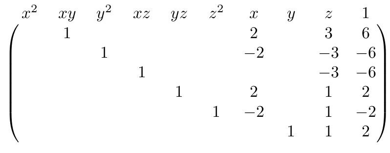
Interpreting the rows as polynomials again, we get the following set $G_2$.\begin{align*}G_2 = \{&xy + 2x + 3z + 6, \\&y^2 – 2x – 3z – 6, \\&xz – 3z – 6, \\&yz + 2x + z + 2, \\&z^2 – 2x + z – 2, \\&y + z + 2\}\end{align*}
Removing redundancies
Some of the elements in $G_2$ are redundant for the ideal $\langle G_2 \rangle$. For example, $\langle G_2 \rangle$ and the ideal spanned by $G_2 \setminus \{xy + 2x + 3z + 6\}$ are the same: We can “build” $(xy + 2x + 3z + 6) = x(y + z + 2) – (xz – 3z – 6)$ from other polynomials in $G_2$.
Removing all redundant elements like this, we end up with $G’_2$.\begin{align*}G’_2 = \{&xz – 3z – 6, \\&z^2 – 2x + z – 2, \\&y + z + 2\}\end{align*}
Checking the result
The burning question: Is $G’_2$ a Gröbner basis for $\langle \mathcal{F} \rangle$? Let’s start applying the Buchberger criterion by building S-Polynomials.
$$\text{S-Poly}(xz – 3z – 6, z^2 – 2x + z – 2) = 2x^2 + 2xy + 3xz + 3yz + 6x + 6y =: g_0$$
Polynomial division of $g_0$ by $G’_2$ leaves remainder $2x^2 – 4x – 6z – 12$. This is not 0, meaning that $G’_2$ is not a Gröbner basis! Bummer. Let’s try the same steps with a bigger Macaulay matrix, going to degree 3.
Raising the degree for the Macaulay matrix
The Macaulay matrix of degree 3 for our system of polynomials $\mathcal{F}$ looks as follows.
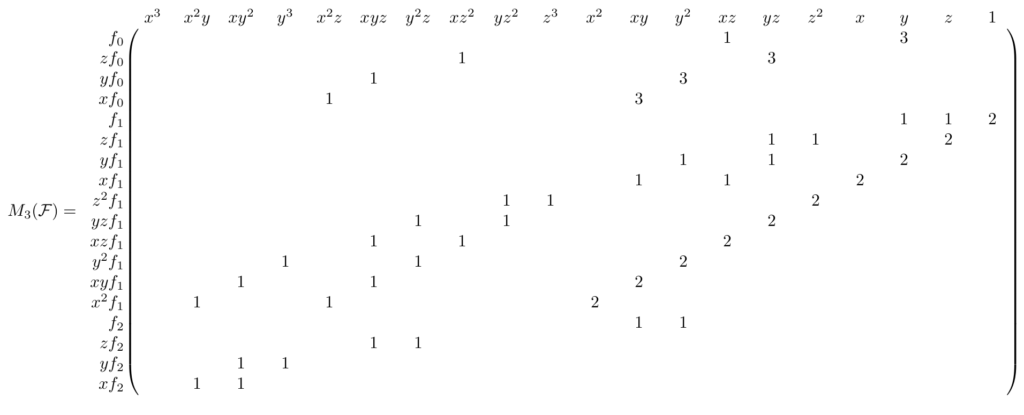
Wow, this has grown! And no wonder: the number of monomials below degree $d$ for a fix number of variables – 3 in our case – grows factorially with $d$. Anyway, the triangulated matrix (with all zero-rows removed) looks a little like this:
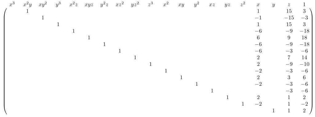
The rows of this matrix correspond to the polynomials in set $G_3$.
\begin{alignat*}{4}G_3 = \{&x^2y + 10x + 15z + 30, &\qquad&xy^2 – 10x – 15z – 30, \\&y^3 + 10x + 15z + 30, &&x^2z – 6x – 9z – 18, \\&xyz + 6x + 9z + 18, &&y^2z – 6x – 9z – 18, \\&xz^2 – 6x – 3z – 6, &&yz^2 + 2x + 7z + 14, \\&z^3 + 2x – 9z – 10, &&x^2 – 2x – 3z – 6, \\&xy + 2x + 3z + 6, &&y^2 – 2x – 3z – 6, \\&xz – 3z – 6, &&yz + 2x + z + 2, \\&z^2 – 2x + z – 2, &&y + z + 2\}\end{alignat*}
Again, we remove redundant polynomials, resulting in $G’_3$. This is only one element bigger than $G’_2$! But this one missing element did the trick: $G’_3$ is a Gröbner basis, spanning the same ideal as $\mathcal{F}$.
\begin{align*}G’_3 = \{&x^2 – 2x – 3z – 6, \\&xz – 3z – 6, \\&z^2 – 2x + z – 2, \\&y + z + 2\}\end{align*}
Note: $G_3$ is also a Gröbner basis for $\langle \mathcal{F} \rangle$, but $G’_3$ is the (unique) reduced Gröbner basis.
The Degree of Regularity
The highest degree of any of the elements in $\mathcal{F}$ is $2$. The same is true for its Gröbner basis $G’_3$. However, in order to compute $G’_3$ from $\mathcal{F}$, we needed to work with polynomials of degree $3$ – the Macaulay matrix $M_2(\mathcal{F})$ of degree 2 did not suffice.
Even though this is not the formal definition, the degree of regularity is the lowest degree for which triangularizing the Macaulay matrix results in a Gröbner basis.
Except in the special case of regular systems, computing the degree of regularity is as hard as computing the Gröbner basis itself – even using more advanced algorithms like F₄ or F₅. This is quite annoying when you want to use the degree of regularity to determine how hard a Gröbner basis computation might get! Luckily, many polynomial systems encountered “in the wild” are in fact regular.
Please note that the degree of regularity allows deriving an upper bound for the complexity of computing a Gröbner basis. Arguing that the compution is difficult for some system by only talking about the degree of regularity is a great faux-pas! If the system behaves like a random one, the upper bound is tight and the argument stands.
Playtime! – Sagemath Code
def all_monoms_upto_deg(ring, d):
    all_monoms = set()
    last_monoms = [ring(1)]
    for i in range(d):
        all_monoms.update(last_monoms)
        last_monoms = [l*v for l in last_monoms for v in ring.gens()]
    all_monoms.update(last_monoms)
    return sorted(all_monoms)[::-1]

def macaulay_matrix(polys, d):
    ring = polys[0].parent()
    columns = all_monoms_upto_deg(ring, d)
    mm_pols = []
    for p in polys:
        factors = [f for f in columns if f.lm()*p.lm() in columns]
        factors = factors[::-1] # original polynomial in highest possible row
        mm_pols += [f*p for f in factors]
    mm_rows = [[p.monomial_coefficient(c) for c in columns] for p in mm_pols]
    return matrix(mm_rows)

def gauss_elimination(A):
    A = copy(A)
    nrows, ncols = A.nrows(), A.ncols()
    for c in range(ncols):
        for r in range(nrows):
            if A[r,c] and not any(A[r,i] for i in range(c)):
                a_inverse = ~A[r,c]
                A.rescale_row(r, a_inverse)
                for i in range(nrows):
                    if i != r and A[i,c]:
                        minus_b = -A[i,c]
                        A.add_multiple_of_row(i, r, minus_b)
                break
    empty_rows = [i for i in range(nrows) if not any(A.row(i))]
    A = A.delete_rows(empty_rows)
    A = matrix(sorted(A)[::-1])
    return A

def polynomial_division(f, divisors):
    f_original = f
    quotients = [0]*len(divisors)
    rem = 0
    while f != 0:
        i = 0
        division_occured = False
        while i < len(divisors) and not division_occured:
            divisable = False
            try:
                divisable = divisors[i].lt().divides(f.lt())
            except NotImplementedError as e:
                pass # _beautiful_ solution
            if divisable:
                q, _ = f.lt().quo_rem(divisors[i].lt())
                quotients[i] += q
                f = f - q * divisors[i]
                division_occured = True
            else:
                i += 1
        if not division_occured:
            r = f.lt()
            rem += r
            f -= r
    assert f_original == sum([q*d for q, d in zip(quotients, divisors)]) + rem
    return quotients, rem

def interreduce(polys):
    i = 0
    while i < len(polys):
        reductee = polys[i]
        polys_wo_reductee = [p for p in polys if p != reductee]
        _, rem = polynomial_division(reductee, polys_wo_reductee)
        if not rem:
            polys = polys_wo_reductee
            i = 0
        else:
            i += 1
    return polys

def s_poly(f, g):
    l = f.lm().lcm(g.lm())
    factor_f = l // f.lt()
    factor_g = l // g.lt()
    return factor_f * f - factor_g * g

def buchberger_criterion(gb):
    for j in range(len(gb)):
        for i in range(j):
            s = s_poly(gb[i], gb[j])
            _, rem = polynomial_division(s, gb)
            if rem:
                return False
    return True

if __name__ == "__main__":
    ring.<x,y,z> = GF(101)[]
    polys = [x*z + 3*y, y + z + 2, x*y + y^2]
    print(f"Ring: {ring}")
    print(f"Input polynomials:\n{polys}")
    d = 0
    is_gb = False
    while not is_gb:
        columns = vector(all_monoms_upto_deg(ring, d))
        mm = macaulay_matrix(polys, d)
        ge = gauss_elimination(mm)
        gb = [row * columns for row in ge]
        gb_red = interreduce(gb)
        quos_rems = [polynomial_division(p, gb_red) for p in polys]
        rems = [r for _, r in quos_rems]
        is_gb = buchberger_criterion(gb_red) and not any(rems)

        print(f"\n––– Degree {d} –––")
        print(f"Macaulay matrix:\n{mm}")
        print(f"Echelon row-reduced Macaulay matrix:\n{ge}")
        print(f"Polynomials in echelon row-reduced Macaulay matrix:\n{gb}")
        print(f"Without redundancies:\n{gb_red}")
        print(f"Is Gröbner Basis: {is_gb}")
        if not is_gb: d += 1
    gb_sage = Ideal(polys).groebner_basis()
    assert sorted(gb_red) == sorted(gb_sage),\
        f"We did not compute the reduced Gröbner basis"
    print(f"Degree of regularity: {d}")