On the Polynomial System of Reinforced Concrete’s Subfunction “Bars”
When designing a symmetric cryptographic primitive, conventional wisdom has it that
- the “simpler” an algebraic model of the primitive, the less secure, and
- a primitive’s algebraic model becomes “complex” by mixing operations from different algebras, like finite fields, or vector spaces.
For example, take the Addition-Rotation-XOR (ARX) design principle. Adding two $n$-bit strings modulo $2^n$ is one of the simplest possible operations for a computer. However, for Gröbner basis analysis of the primitive, we need a polynomial $f^+$ modeling the same operation, and the polynomial’s coefficients need to come from a field. Unfortunately, the field-native addition of two elements from $\mathbb{F}_{2^n}$ corresponds to XOR. Representing addition of bit strings modulo $2^n$ requires a polynomial of quite high degree. That’s bad for algebraic cryptanalysis.
Another consequence is that ARX primitives are no suitable candidates when low arithmetic complexity is required, which includes most modern Zero-Knowledge Proof Systems. This is one of the reasons why hash functions like Rescue Prime [1,3] and Poseidon [2] have emerged: simple algebraic representability. Roughly summarized, they’re designed to have polynomial representation simple enough – meaning few and low-degree polynomials – for efficient use in Zero-Knowledge Proof Systems, but complex enough to thwart the most efficient algebraic analysis methods. Most notably, all operations can be easily modeled over the same finite field, counter to the second piece of “conventional wisdom” above.
Reinforced Concrete’s Subfunction “Bars”
The recently proposed Plookup-friendly Hash function “Reinforced Concrete” [4] can be seen as a mix of those two paradigms: all subfunctions are either linear or can be expressed as low-degree polynomials over some finite field, but not always over the same field. The algebraically most interesting subfunction, “Bars,” is the primary defense against Gröbner basis attacks. It essentially consists of the following steps:
- Variable-base decomposition of the input
- Conditional application of a small S-Box
- Variable-base composition
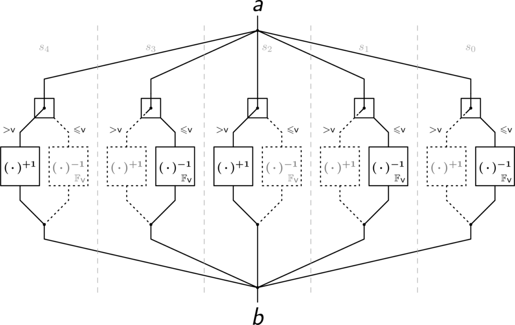
Variable-base decomposition Decomposition takes a field element and returns a tuple. Giving intuition with an example, take a = 318. Fix-base decomposing a with base 10, we can write $\boldsymbol{\textsf{a}} = 3\cdot(10\cdot 10) + 1\cdot(10) + 8$, and decomposition thus results in $(3, 1, 8)$. Choosing a variable base instead, say $(s_2, s_1, s_0) = (13, 9, 12)$, we can write $\boldsymbol{\textsf{a}} = 2\cdot(9\cdot 12) + 8\cdot(12) + 6$, and this variable-base decomposition thus results in $(2, 8, 6)$. More formally, given base $(s_{n-1}, \dots, s_0)$, we can decompose like this: $$\begin{align*}a_0 &= \boldsymbol{\textsf{a}}\bmod{s_0},\\a_i &= \frac{\boldsymbol{\textsf{a}}-\sum_{j<i}a_j\prod_{k<j}s_k}{\prod_{j<i}s_j}\bmod{s_i}.\end{align*}$$
Conditional S-Box application A permutation is applied to each $a_i$ that is smaller or equal to a threshold value $\textsf{v}$. For the Reinforced Concrete instance this post is concerned with, $\textsf{v}$ is prime, and the permutation amounts to inversion of $s_i$ as an element of finite field $\mathbb{F}_\textsf{v}$. Picking up the example from above, let $\textsf{v} = 7$ and $(a_2, a_1, a_0) = (2, 8, 6)$. The S-Box is applied to $a_2$ and $a_0$, but not to $a_1$, because it is greater than $\textsf{v}$. The multiplicative inverse of $2$ in $\mathbb{F}_7$ is $4$, that of $6$ is $6$. The result is $(b_2, b_1, b_0) = (4, 8, 6)$. A more formal description of this step is $$b_i=\textsf{S-Box}(a_i) = \begin{cases}a_i &\text{ if } a_i > \textsf{v},\\\textsf{inv}_{\mathbb{F}_\textsf{v}}(a_i) &\text{ if } a_i \leqslant \textsf{v}.\end{cases}$$
Variable-base composition Going back from a tuple of elements to one field element, composition is the inverse of the first step. Finishing up the running example, composition gives $\boldsymbol{\textsf{b}} = 4\cdot(9\cdot 12) + 8\cdot(12) + 6 = 534$. Formally, we have $$\boldsymbol{\textsf{b}} = \sum_i b_i \prod_{j<i} s_j.$$
A Polynomial System for “Bars”
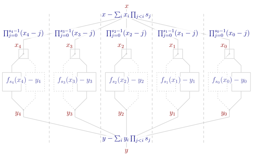
Building a polynomial model for Bars is most straightforwardly done by modeling each of the steps. Let’s start with the decomposition of input $x$, where $x$ is a variable. We introduce one new variable for each decomposition-basis element $s_i$. Decomposition can then be written as $x -\! \sum_i x_i \prod_{j<i}s_j$, which is a linear polynomial. However, this polynomial does not guarantee that $x_i$ can only take values in the range $[0, s_i[$. We therefore need to add additional polynomial constraints that can only be satisfied if $x_i$ is in the specified range. The polynomial we’re looking for is $\prod_{j=0}^{s_i-1}(x_i – j)$: it is zero if and only if $0 \leqslant x_i < s_i$. Summarizing, we introduce $n$ polynomials, one of degree $s_i$ for each element in the decomposition’s variable base.
For composition, we introduce another $n$ many variables $y_i$ for the output of the S-Boxes, and variable $y$ for the output of Bars. Then, composition can be written as $y -\! \sum_i y_i \prod_{j < i} s_j$, much like before. The condition $0 \leqslant y_i \leqslant s_i$ will be implicitly ensured by the next and last step.
All that remains is linking the $x_i$ with the $y_i$ by modeling the conditional application of the S-Box. I have tried cleverly applying the Bézout identity, but the resulting polynomials were of considerably higher degree than just bluntly applying Lagrange interpolation. As a result, getting the polynomials for this step is easy but not pretty: create a list with $s_i$ many entries $(i, \textsf{S-Box}(i))$ and univariably interpolate this list using variable $x_i$, resulting in polynomial $f_{s_i}(x_i)$. Then, $f_{s_i}(x_i) – y_i$ correctly relates variables $x_i$ and $y_i$. In total, this means adding another $n$ polynomials of degrees $s_i – 1$, respectively.
Computing the Gröbner Basis
Summarizing the polynomial system, we have introduced $2n+2$ variables, as well as $2n+2$ polynomials. Two of these polynomials – composition and decomposition – are linear, and for each $s_i$, we have one polynomial of degree $s_i$ and one of degree $s_i – 1$.
Assuming this polynomial system is a regular sequence – and my experiments indicate this to be the case – the Macaulay bound helps with upper bounding the complexity of the Gröbner basis computation. For a set of polynomials $\{f_0, \dots, f_{m-1}\}$, the Macaulay bound is $$1 + \sum_i \deg(f_i) – 1.$$ Plugging in the numbers of the just built polynomial system modeling subfunction Bars, the Macaulay bound is $1 + \sum_i s_i – 1 + \sum_i s_i – 2 = 1 – 3n + 2\sum_i s_i$. The suggested parameters for the BN254 curve are $n=27$ and each of the $s_i$ lies in the range $[668, 703]$. This means the Macaulay bound is enormous: $37408$ to be exact.
Computing the Gröbner basis for a regular sequence that has a big Macaulay bound is, generally speaking, very hard. Unfortunately, we currently only have worst-case bounds, but no way to (tightly) estimate the complexity of computing the Gröbner basis for a concrete polynomial system. Instead, we perform tests on toy examples and see if everything holds up.
Let’s build the polynomial system for Bars based on some toy-sized parameters: $p=47$, $v=5$, $n=2$, and $s_0=s_1=7$. We’ll have to deal with $6$ variables and $6$ equations, and the Macaulay bound for the resulting system is $23$. This is not nothing, but it’s also not very big: the polynomial system of 6 full rounds of Poseidon (with state size 2) has the same Macaulay bound, and the system for 5 rounds of Rescue (also state size 2) has comparable Macaulay bound $21$. For reference, I’ve put the resulting polynomial system $\mathcal{F}^{[7,7]}_{(47,5)}$ below, but reading it is not necessary for the rest of this post.
Computing the associated Gröbner basis (in degrevlex order) is surprisingly fast, and the degree of the highest degree polynomial appearing in any intermediary step is $7$. That’s not even close to the Macaulay bound! So why is the computation so much easier than anticipated? There are some further observations to be made, for which we first need to go on a slight tangent.
Vectors of Origin
For polynomial sequence $\mathcal{F} = (f_0, \dots, f_{m-1})$, any element $g$ from its Gröbner basis is a (non-linear) combination of the input elements: $g = \sum_i h_i\cdot f_i$ or, using vector notation, $g = \boldsymbol{h}\cdot\mathcal{F}$. I call $\boldsymbol{h}$ the vector of origin for $g$ because it tells us where $g$ originates from in relation to $\mathcal{F}$. The set of vectors of origin describing the entire Gröbner basis is packed with information, and not all of it is easy to interpret. But something that’s glaringly obvious in any vector of origin is a zero-entry. A zero in position $i$ in vector of origin $\boldsymbol{h}$ means that $f_i$ was unnecessary for computing $g$.
I’ve used the tool VooDoo to compute the vectors of origin for the polynomial system $\mathcal{F}^{[7,7]}_{(47,5)}$. For clarity of reading, any big polynomial is replaced by $\bullet$. Here’s what the vectors look like:
$$\begin{align} &(1, {\small 0}, {\small 0}, {\small 0}, {\small 0}, {\small 0}),\\ &({\small 0} , \bullet, \bullet, {\small 0}, {\small 0}, {\small 0}),\\ &({\small 0} , \bullet, \bullet, {\small 0}, {\small 0}, {\small 0}),\\ &({\small 0} , \bullet, \bullet, {\small 0}, {\small 0}, {\small 0}),\\ &({\small 0} , {\small 0}, {\small 0}, \bullet, \bullet, {\small 0}),\\ &({\small 0} , {\small 0}, {\small 0}, \bullet, \bullet, {\small 0}),\\ &({\small 0} , {\small 0}, {\small 0}, \bullet, \bullet, {\small 0}),\\ &({\small 0} , {\small 0}, {\small 0}, {\small 0}, {\small 0}, 1) \end{align}$$
See the pattern? It appears that computing the Gröbner basis for $\mathcal{F}^{[7,7]}_{(47,5)}$ can be reduced to computing on multiple smaller systems. After all, the polynomials describing one S-Box are pretty much completely independent from the polynomials describing another S-Box. Dividing and conquering is a strategy that is usually impossible for computing a Gröbner basis, but in this specific case, it’s back on the table: the Macaulay bound for the sub-system describing one S-Box is $1+ s_i – 1 + s_i – 2$, amounting to $12$ in our toy example. This doesn’t fully explain the discrepancy to the observed highest degree of $7$ yet, suggesting that more interesting riddles are waiting to be solved.
Above analysis doesn’t mean that using subfunction Bars is unsuitable for preventing Gröbner basis attacks. However, looking at the entire polynomial system and relying on the complexity upper bound for the Gröbner basis computation implied by the Macaulay bound is probably too optimistic.
References
- Aly, A., Ashur, T., Ben-Sasson, E., Dhooghe, S., Szepieniec, A.: Design of Symmetric Primitives for Advanced Cryptographic Protocols. IACR ToSC 2020(3), 1–45(2020)
- Grassi, L., Khovratovich, D., Rechberger, C., Roy, A., Schofnegger, M.: Poseidon: A New Hash Function for Zero-Knowledge Proof Systems. In: USENIX Security. USENIX Association (2020)
- Szepieniec, A., Ashur, T., Dhooghe, S.: Rescue-Prime: a standard specification (SoK). Cryptology ePrint Archive, Report 2020/1143 (2020), https://eprint.iacr. org/2020/1143
- Barbara, M., Grass, L., Khovratovich, D., Lueftenegger, R., Rechberger, C., Schofnegger, M., Walch, R.: Reinforced Concrete: Fast Hash Function for Zero Knowledge Proofs and Verifiable Computation. Cryptology ePrint Archive, Report 2021/1038 (2021), https://eprint.iacr.org/2021/1038
Appendix: The Polynomial System
Below, you can find the polynomial system for the toy-sized parameters from above. Note how the polynomials corresponding to the S-Boxes are identical, which is due to $s_0 = s_1$ and does not generally hold. The same is true for the polynomials ensuring $0 \leqslant x_i < s_i$. However, the similarities between the decomposition polynomial and the composition polynomial is inherent.
$$\mathcal{F}^{[7,7]}_{(47,5)} = \begin{cases} x – 7x_1 – x_0 & \text{decomposition}\\[0.5em] x_0^7 – 21x_0^6 – 13x_0^5 + 17x_0^4 – 21x_0^3 + 22x_0^2 + 15x_0 & 0 \leqslant x_0 < s_0\\[0.5em] 18x_0^6 + 4x_0^5 – 15x_0^4 – 17x_0^3 – 15x_0^2 – 21x_0 – y_0 & y_0 = \textsf{S-Box}(x_0)\\[0.5em] x_1^7 – 21x_1^6 – 13x_1^5 + 17x_1^4 – 21x_1^3 + 22x_1^2 + 15x_1 & 0 \leqslant x_1 < s_1\\[0.5em] 18x_1^6 + 4x_1^5 – 15x_1^4 – 17x_1^3 – 15x_1^2 – 21x_1 – y_1 & y_1 = \textsf{S-Box}(x_1)\\[0.5em] y – 7y_1 – y_0 & \text{composition} \end{cases}$$
The associated reduced Gröbner basis reads as follows.
$$\mathcal{G}^{[7,7]}_{(47,5)} = \begin{cases} x – 7x_1 – x_0 & \text{decomposition}\\[0.5em] \left. \begin{aligned} &x_0^2 – y_0^2 – 5x_0 + 5y_0\\[0.5em] &x_0y_0^2 – y_0^3 – 5x_0y_0 + 5y_0^2 + 6x_0 – 6y_0\\[0.5em] &y_0^5 – 16y_0^4 – 5y_0^3 + 10x_0y_0 – 16y_0^2 – 19x_0 – 2y_0 \end{aligned} \right\} & \textsf{S-Box } s_0 \\[0.5em] \left. \begin{aligned} &x_1^2 – y_1^2 – 5x_1 + 5y_1\\[0.5em] &x_1y_1^2 – y_1^3 – 5x_1y_1 + 5y_1^2 + 6x_1 – 6y_1\\[0.5em] &y_1^5 – 16y_1^4 – 5y_1^3 + 10x_1y_1 – 16y_1^2 – 19x_1 – 2y_1\\[0.5em] \end{aligned} \right\} & \textsf{S-Box } s_1 \\[0.5em] y – 7y_1 – y_0 & \text{composition} \end{cases} $$
Leave a Reply